3 Use Case 1: Above Ground Carbon & Visualising Uncertainty
Kew Science are carrying out detailed empirical studies at Wakehurst to improve understanding of the amount of carbon stored in particular habitats and the factors that influence it. The case study in LIMMMA was to compare and contrast models of carbon storage, bringing in refinements from the Kew work in ‘real time’, being able to visualise uncertainties in both data sets and models. We aimed to utilise these latest empirical insights in LIMMMA to support the creation of models of carbon storage that could be scaled up from local to national level; complementing and comparing with those models and outputs currently in use. Outputs could be examined alongside existing estimates of carbon storage making both the uncertainties involved and limits to scaling clear. The principles apply to many other ongoing initiatives to enhance understanding of carbon storage.
In the following walkthrough we demonstrate how the above ground carbon models were created and tested using LIMMMA. If you prefer a video walkthrough you can watch the video below. Otherwise, continue to the next section which provides the same content as the video in the form of text and slides. For a technical discussion of this work download the full report.
3.1 Methodologies and Datasets
We worked in partnership with Kew Science to develop a workflow for generating and improving geospatial estimates of the amount of carbon stored above ground in the natural landscape which met the following requirements:
- Informed by new data, equations (e.g. allometry) and methodologies as they emerge from ongoing research.
- Scaleable from local to national using open access national datasets.
- Supports comparison of different models across multiple scales.
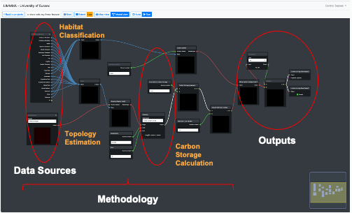
The data and methods adopted are summarised in the following diagram.
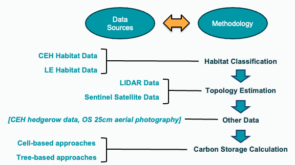
Habitat Classification: Two options for generating the habitat basemap for carbon estimates were imported – one from the UK Centre for Ecology and Hydrology (UKCEH) and the other from Living England (LE).
Topology Estimation: LIDAR and Sentinel Satellite imagery provided the two options for topology estimation which, depending on the model, were used to determine tree canopy height or feature height respectively.
Other Data: Additional data included UKCEH hedgerows and OS 25cm arial photography (which was used with the AI component).
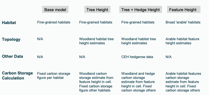
These data were variously used in different methods of carbon storage calculation using a cell-based approach. The four methodologies listed below build on each other iteratively to progress towards a more precise estimate of carbon storage generated by increasingly complex models with potential for continuous improvement.
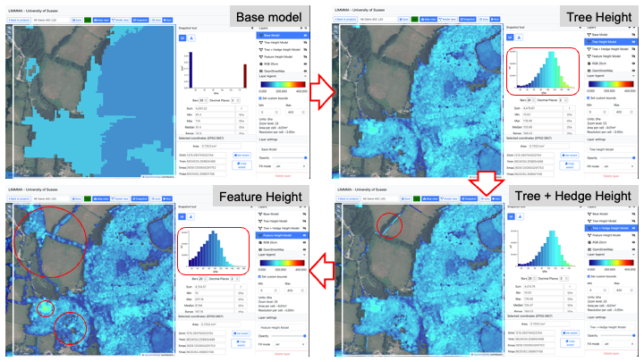
In the image below we can see how each model progressively improves the fidelity of carbon estimate maps by variously increasing their resolution and coverage.
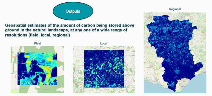
And here is an example of the outputs from the model in LIMMMA map view at different scales.
The following section describes how each of these models was built and how the outputs were created and analysed to draw conclusions about the different levels and locations of uncertainty given the discrepancy between two equally valid data sources.
3.2 Implementing models
Each model was built in LIMMMA’s graphical modelling system. The following diagram shows how this is used to connect data, methods and outputs in a single visual interface.
In this section we present a series of step-by-step guides showing you how to reproduce the final feature height model from scratch. Each part of the process is illustrated in slide show format (see below).
Use slide show arrows or your keyboard arrow buttons to move through the slides. Hold down ‘alt’ and click to zoom in on a slide. Use the menu button at the bottom left of each slide show to open up the viewing options where you can see a list of the slides and the option to view in full screen.
3.2.1 Selecting datasets
Having created a new project and set our desired extent, we can open the model view and start building. At first, you will be presented with a blank screen with no visible controls. Don’t worry, the first thing to do is to add the various components you want to include in your model. This is done by simply right clicking the screen and selecting from a list of various types of components (see below). Datasets will include whatever your team has imported into your LIMMMA workspace. In addition to datasets there are numerous components for transforming inputs from those datasets in various ways and converting them into outputs for use in map view or in other models.
The first step in building our model is to add to the model the various datasets we need. This model only uses two:
- Boolean dataset from the Living England Land Cover classification.
- Numerical dataset of feature height derived from LIDAR imaging.
Let’s first add these to the model.
It is important to understand at this point that, when a dataset is added to a model it is converted to a raster format with cell dimensions adjusted to match the zoom level of the project. So whether it is a categorical, boolean or numerical dataset each dataset will share the same resolution. The zoom level is is determined according to the extent chosen when the project was created. However, the extent can also be adjusted from model view if you want to change to scale at which the model is run. This can be very useful when you need to run a model at different scales without having to rebuild it every time.
3.2.2 Combining datasets
Next we need to generate the broader categories of land cover class that we will use in the model. The first is a collection of land cover classes with little or no vegetation. This will not be computed with the feature height data but simply assigned a negligible average carbon density value (i.e. 0.001). The second is a collection of land cover classes that contain vegetation of various kinds and which will be computed with the feature height data and an equation to estimate carbon density based on the height of vegetation.
3.2.3 Transforming data
Having added the datasets and organised the land cover classes we can start to use them to generate carbon storage estimates. The basic principle is to use the land cover categories (‘No vegetation’ and ‘Vegetation’) to mask numerical data that represents an estimate of biomass that can then be converted into an estimate of carbon stored per cell (i.e. per unit area) for each category. For simplicity we count all the land cover classes in the ‘No vegetation’ category as containing no biomass and therefore holding almost no stored carbon so we want to assign each ‘No vegetation’ cell the value 0.001.
The next step is more complex. We now want to use the feature height (spatial numeric data) to estimate the carbon density distribution in all the ‘vegetation’ land cover classes. First we need to mask the feature height data with the ‘vegetation’ category and then we can use an equation to calculate estimates of biomass from the average feature height recorded for each cell. Here is how we do it.
We are not finished with the vegetation category yet. To calculate an estimate of biomass based on the feature height measurements we need to use an equation from the ‘Expression’ component. In this example there are three expressions to choose from but it is possible to create any number of bespoke options using the ‘Expressions’ menu.
Now we have two maps of biomass: one for all land cover classes without vegetation and one for all land cover classes with vegetation. To create a single map for the whole landscape we need to merge these together.
Finally, we need to convert the estimate of biomass into above ground stored carbon (AGC). We will use the ‘Multiply’ and ‘Numeric constant’ components to convert to kg of carbon per m^2 and then into tonnes of carbon per hectare.
3.2.4 Generating outputs
Now we have a model that generates a density map for above ground vegetative carbon we need to translate this into outputs for the map view and for use in other projects.
3.3 Exploring outputs
Switching to ‘Map view’ we can explore the new map layer visually alongside other map layers and also use the ‘Snapshot’ tool to view information for selected areas.
While this carbon density map gives the impression of a highly detailed and accurate estimate of carbon stored in the landscape there is, in fact, one crucial layer of information missing. As it stands, it fails to communicate the various sources, dimensions and locations of uncertainty associated with the estimates of carbon density.
3.4 Visualising Uncertainty
This section explains how LIMMMA can be used to build into the carbon density models a system for visualising uncertainties associated with measurement, modelling parameters, false positives and habitat classification methods. Here we describe the method adopted for calculating combined estimates of uncertainty and how this method is implemented in LIMMMA.
Uncertainty and confidence-level estimation
Our proposed method combines uncertainty and level-of-confidence through a simple framework that combines all sources of uncertainty into one figure, providing a single measure of uncertainty that incorporates degree of confidence. We structure sources of uncertainty into two categories: (i) “data uncertainty”, uncertainty attributable to problems with the data, including measurement errors, natural variation, and missing or otherwise problematic data; and (ii) “methodological uncertainty”, which is primarily driven by our limited confidence in our models. The latter sources of uncertainty are typically signalled qualitatively (e.g. “low confidence”) so this approach attempts to integrate such concerns into a numerical framework.
These differing sources of uncertainty need to be estimated and then propagated appropriately and/or conservatively through a model to capture a realistic approximation of uncertainty that is of some value to a decision-maker. We currently apply these approaches to incorporate uncertainty estimates into the following assessments:
- What is the uncertainty (standard deviation) associated with a measurement of something at a single unit patch of landscape (a single cell in our LIMMMA model, typically varying in size from 1.5 m (field level, zoom 24) to 24 m (regional level, zoom 20).
- What is the uncertainty (standard deviation) associated with the measurement of the total (sum) of something across an extent made up of multiple modelled patches?
- What is the uncertainty (standard deviation) associated with the estimation of the average value of something across an extent made up of multiple modelled patches?
We combine uncertainties under the conservative assumption of independence, adding together the variances of each separate component of uncertainty to estimate the variance of the whole:
- For an individual patch in the model, the standard deviation of the estimate for the patch (uncertainty estimate) is then the square root of this sum.
- For an extent, the uncertainty of the sum of the estimated figure is the square root of the sum of each patch’s total variance.
- The uncertainty of the average (the standard error) is this figure divided by the square root of the number of patches in the extent.
Implementing uncertainty visualisation
In the feature height model shown in the above walkthrough, there are at least four sources of uncertainty which can be estimated and visualised. These are:
- Measurement uncertainty: how much error is involved in the measurement of feature height?
- Parameter uncertainty: how well does the allometric equation predict the relationship between the height of features and the quantity of stored carbon?
- False positives: how likely is it for a “feature” in non-woodland vegetation habitats to be a false positive?
- Habitat disagreement: how confident are we in the classification of each patch of habitat where it has a direct implication for the model?
Through analysis and comparison of the outputs from the models run at different scales, across different extents and using different habitat classification datasets, we produced initial estimates of uncertainty for each of these four sources. These are summarised in the table below.
| Type | Description | Estimate |
|---|---|---|
| Measurement | Measurement of feature height (Lidar terrain, surface). | 1 s.d. = 4% of height (e.g. 60cm on 15m tree). Var = 0.0016 |
| Parameter | Variability around model parameter fit to data due to natural variation. | Parameter fit 1.s.d = +/- 15% multiplier. Var = 0.02225 |
| False positives | Missing data requires interpolation or other assumptions. | False positives on arable, grassland 1 s.d. = 1 tC/ha. Var = 0.1 |
| Habitat disagreement | “Black box” ML model with unpredictable failure modes. | Locations of disagreement in habitat map. 1 s.d. = 60 tC/ha. Var = 3600 |
Each of these sources of uncertainty can be modelled in LIMMMA alongside the carbon storage model to generate a map output which shows not only the distribution of carbon density but also the distribution of uncertainty associated with each estimate for each cell (or patch of land) in the model. This makes it possible to trace not only the sources of uncertainty but also to identify those locations in the landscape where carbon estimates are most prone to error. Let’s see how to create this type of model from scratch.
The first step is to create a new project and to re-built the carbon storage model (this time we will use the alternative habitat classification).
Next we will add the model cluster for measurement and parameter uncertainty.
Now the cluster for false positives.
Finally, we will add the cluster to calculate uncertainty based on habitat disagreement.
Having added model clusters to deal with uncertainty in measurement, parameters, false positives and habitat disagreement we now need to combine these into a composite uncertainty distribution. This is done as follows.
But, what if we want to re-run the model over a larger area or in another location? All we need to do is toggle back to Model view, edit the project extent and re-run the model like this:
Now we have a carbon density map which can be examined in direct comparison with its associated uncertainty distribution. This basic model structure could then be used and improved to test the effects of different assumptions about uncertainty, compare relative uncertainties associated with different data sources and models, or run at various scales and locations to produce new insights.