2  Getting Started

2.1 Making an account

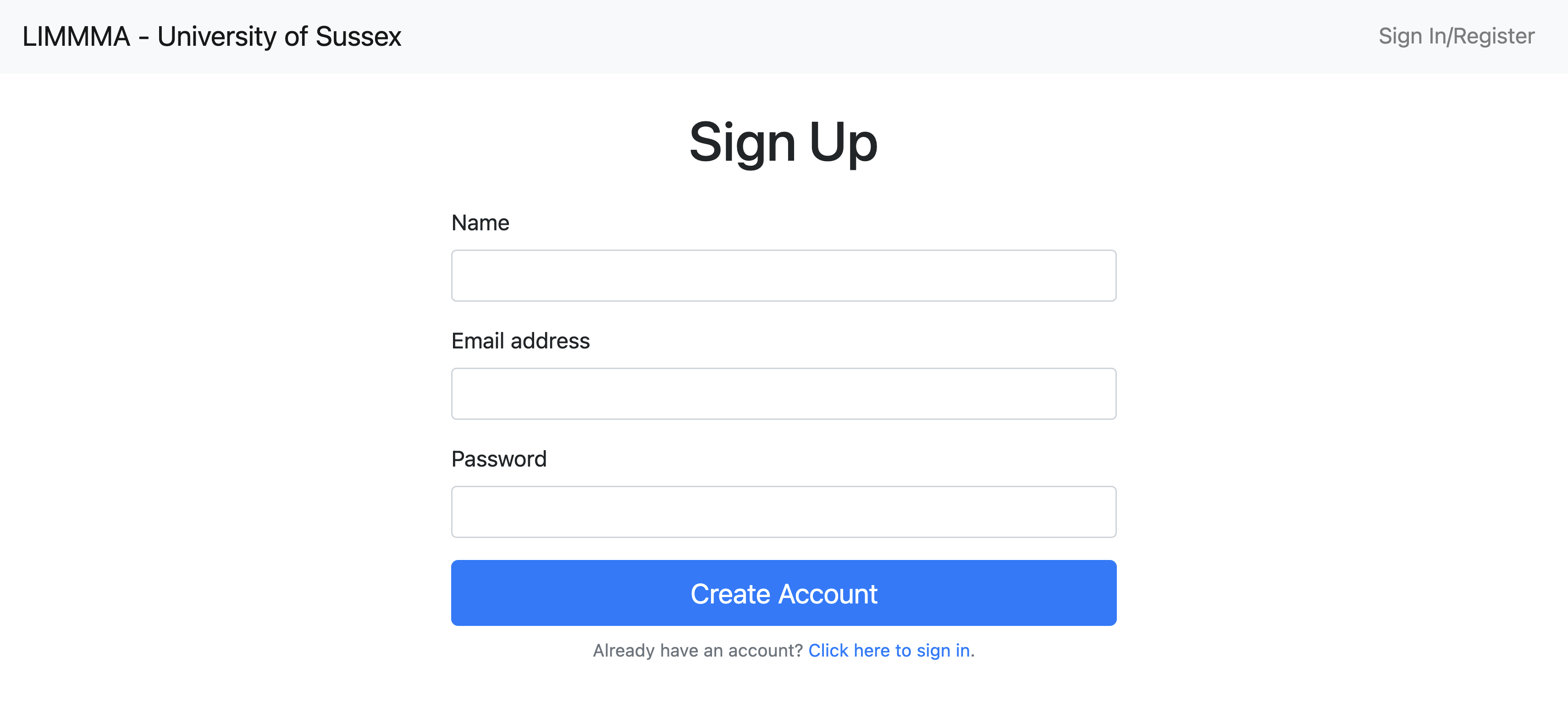
Sign in or sign up to make an account here: https://landscapes.wearepal.ai/

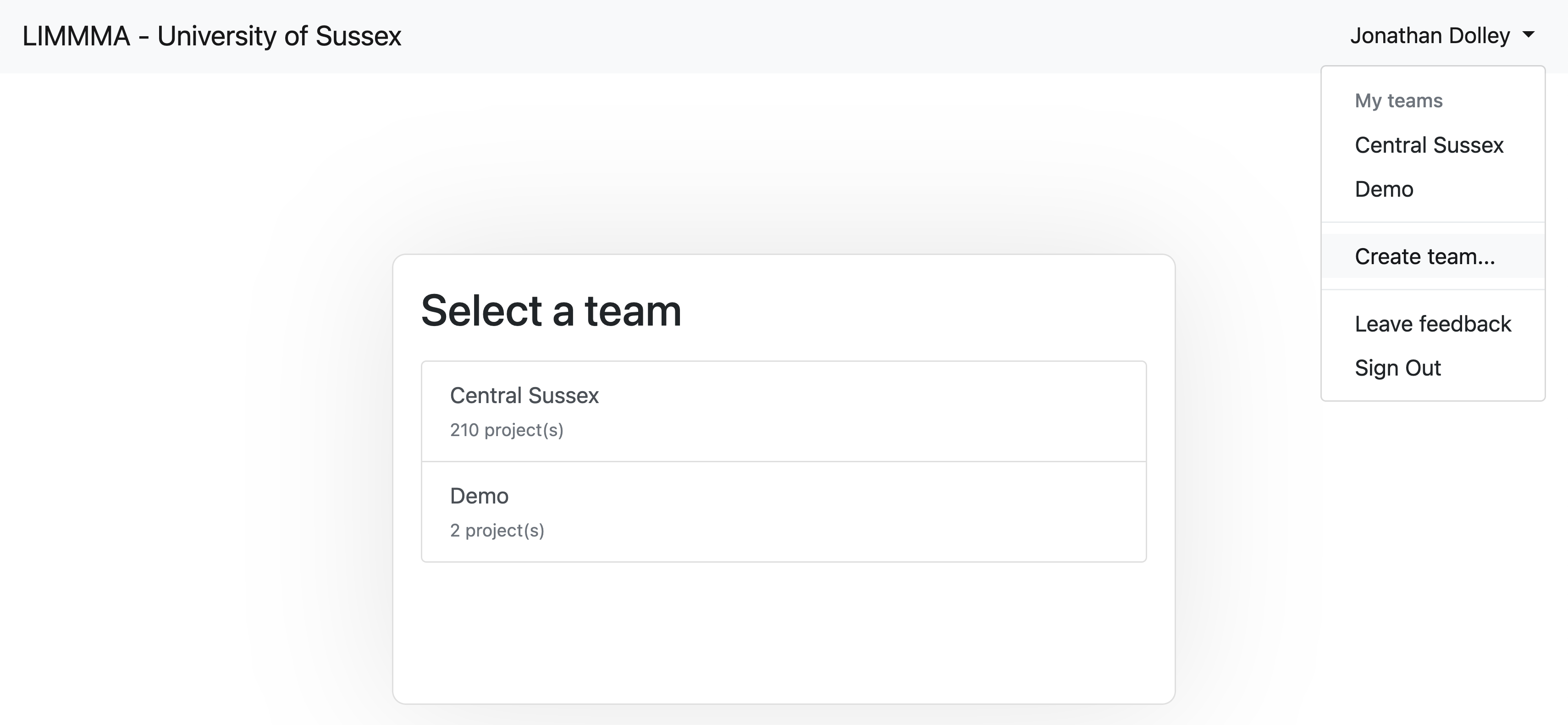
Then select a team or create a new one. You will automatically be added to the “Guest” team where you can view live demo projects. Details of how these live demo projects were created are given in chapters 3 and 5.

2.2 Setting up a new project

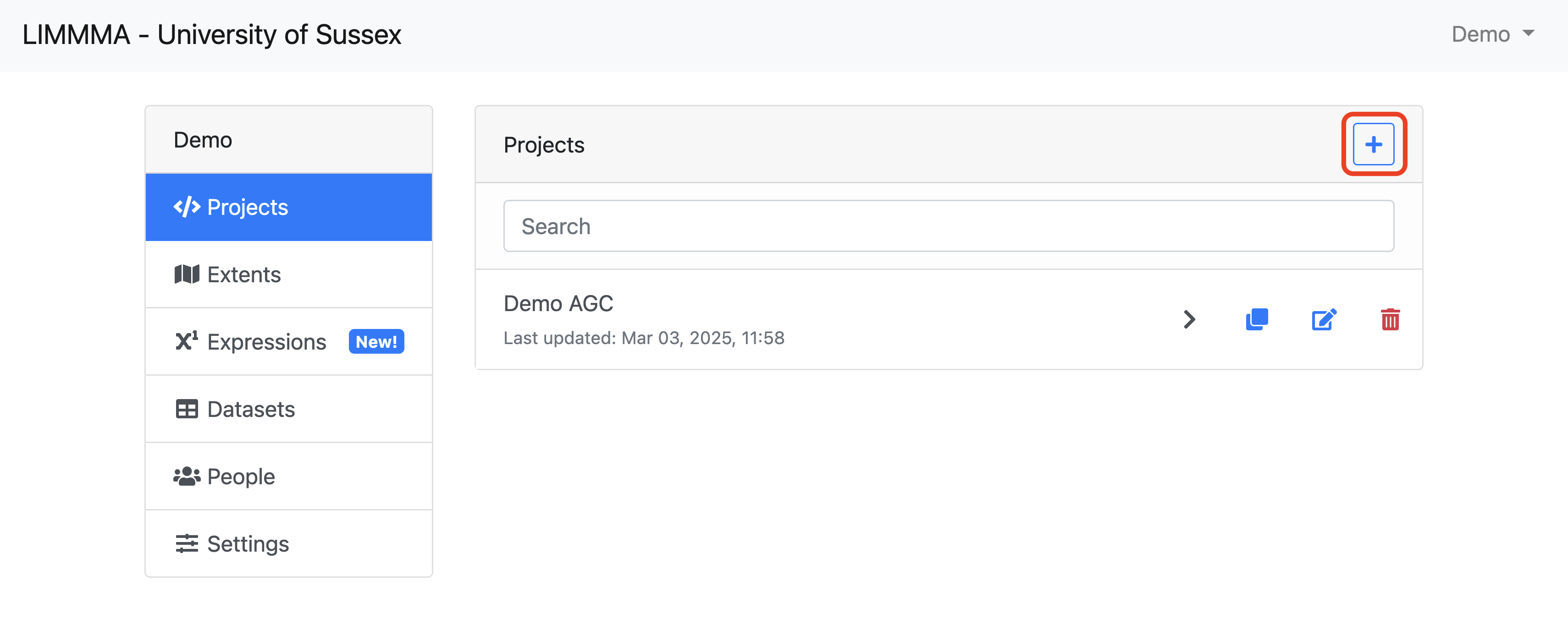
After you have logged in to your team workspace, the first menu you will see is the Project Menu. Click the blue”+” symbol to create a new project.

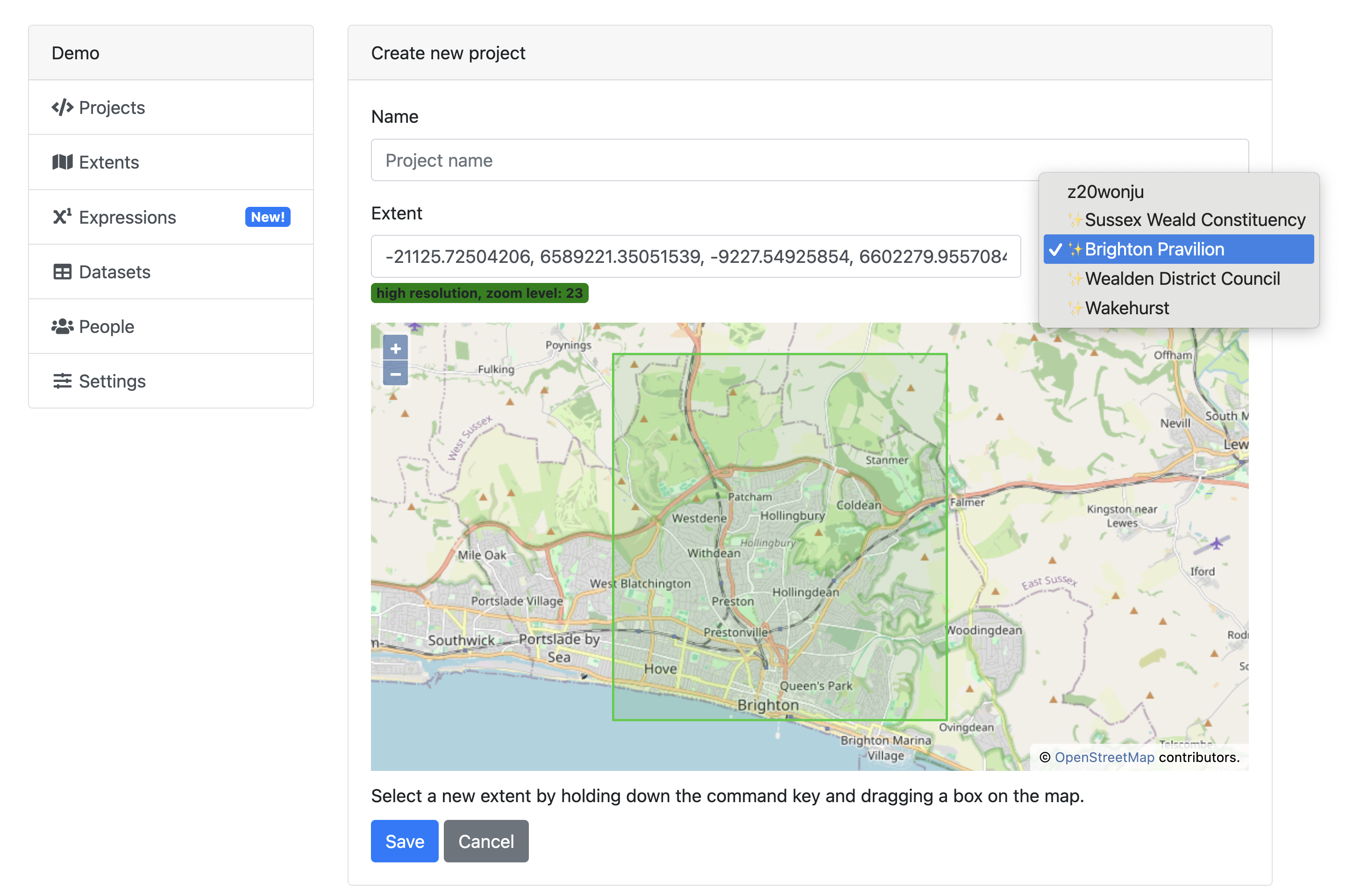
First you will need to select an extent for the project and give the project a name. These can both be changed later if necessary.

2.3 Adding Map Layers

When you open the project, the default view is Map View.

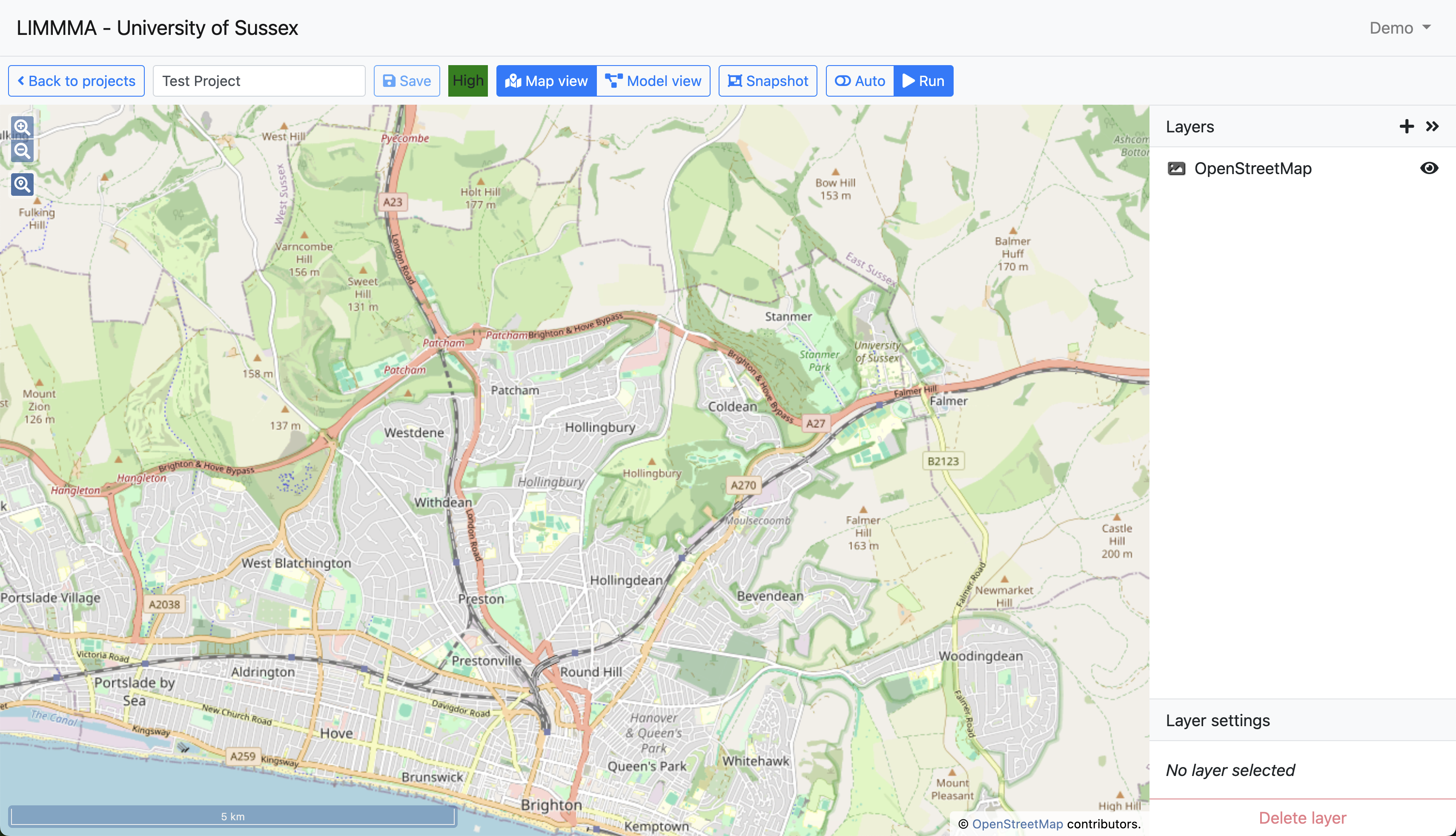
Click the black “+” next to the “Layers” heading to add map layers.

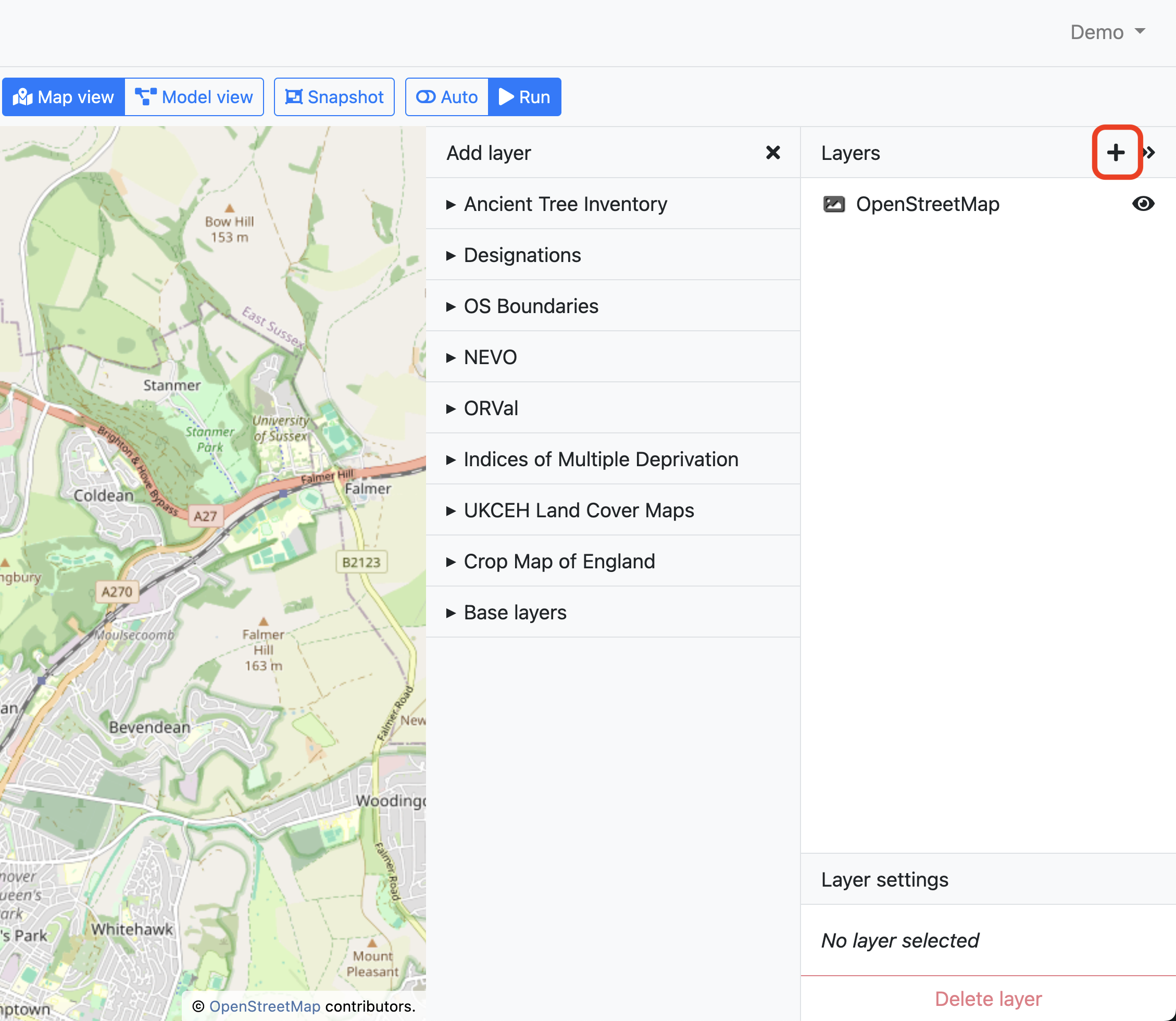
There are a variety of layers available, organised into groups of drop down menus. We will choose one from the “Designations” group.

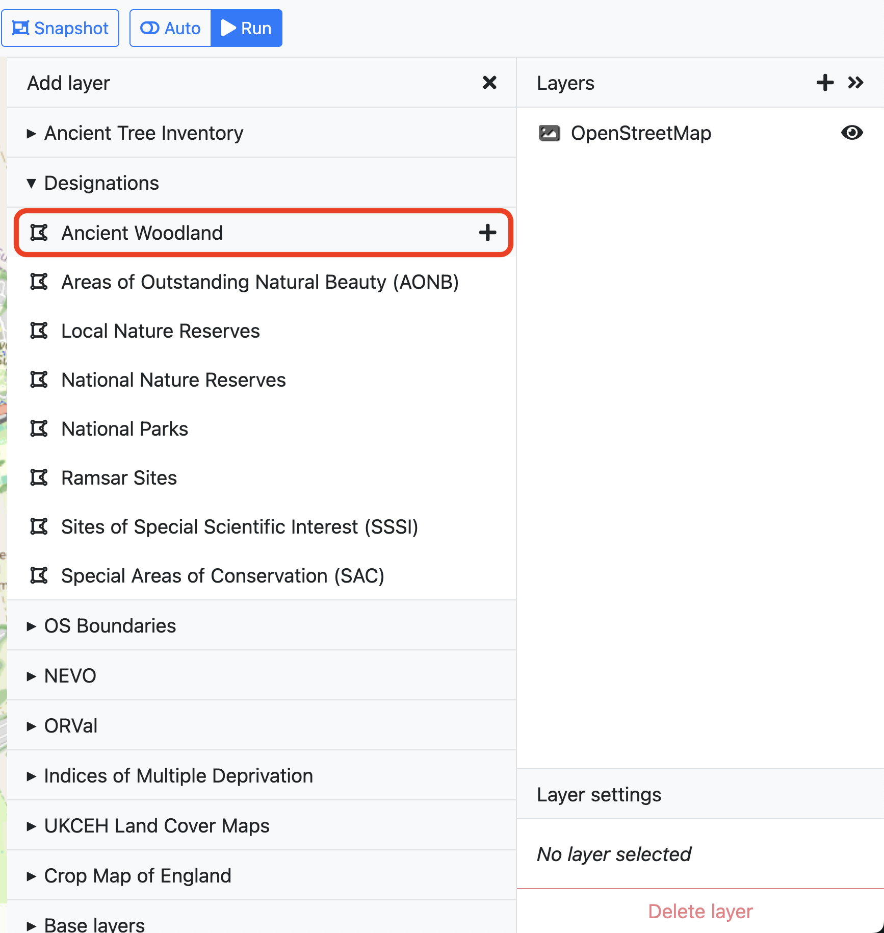
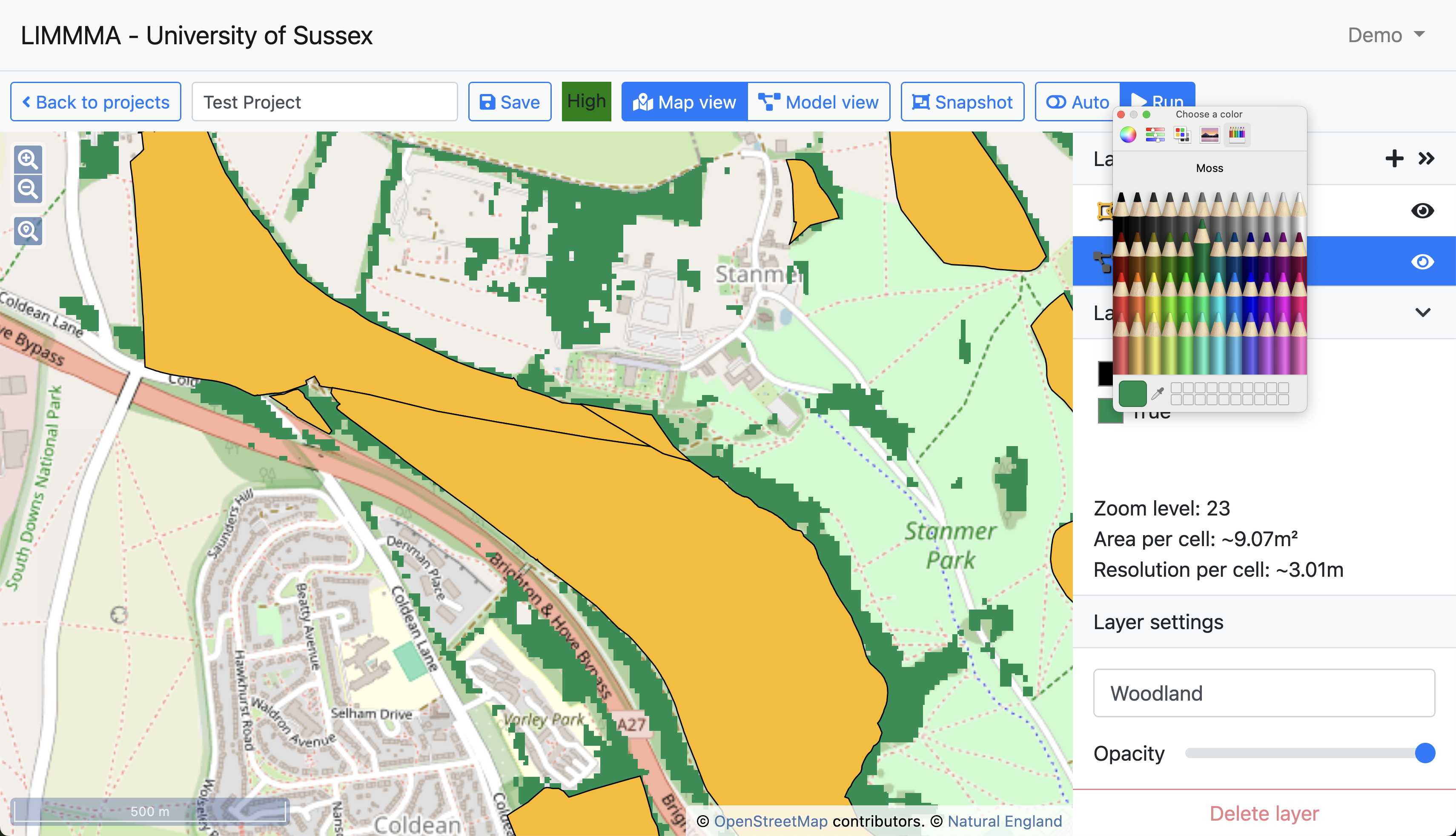
Let’s add “Ancient Woodland” to the map. It now shows up in the layer menu on the right and on the map in orange.

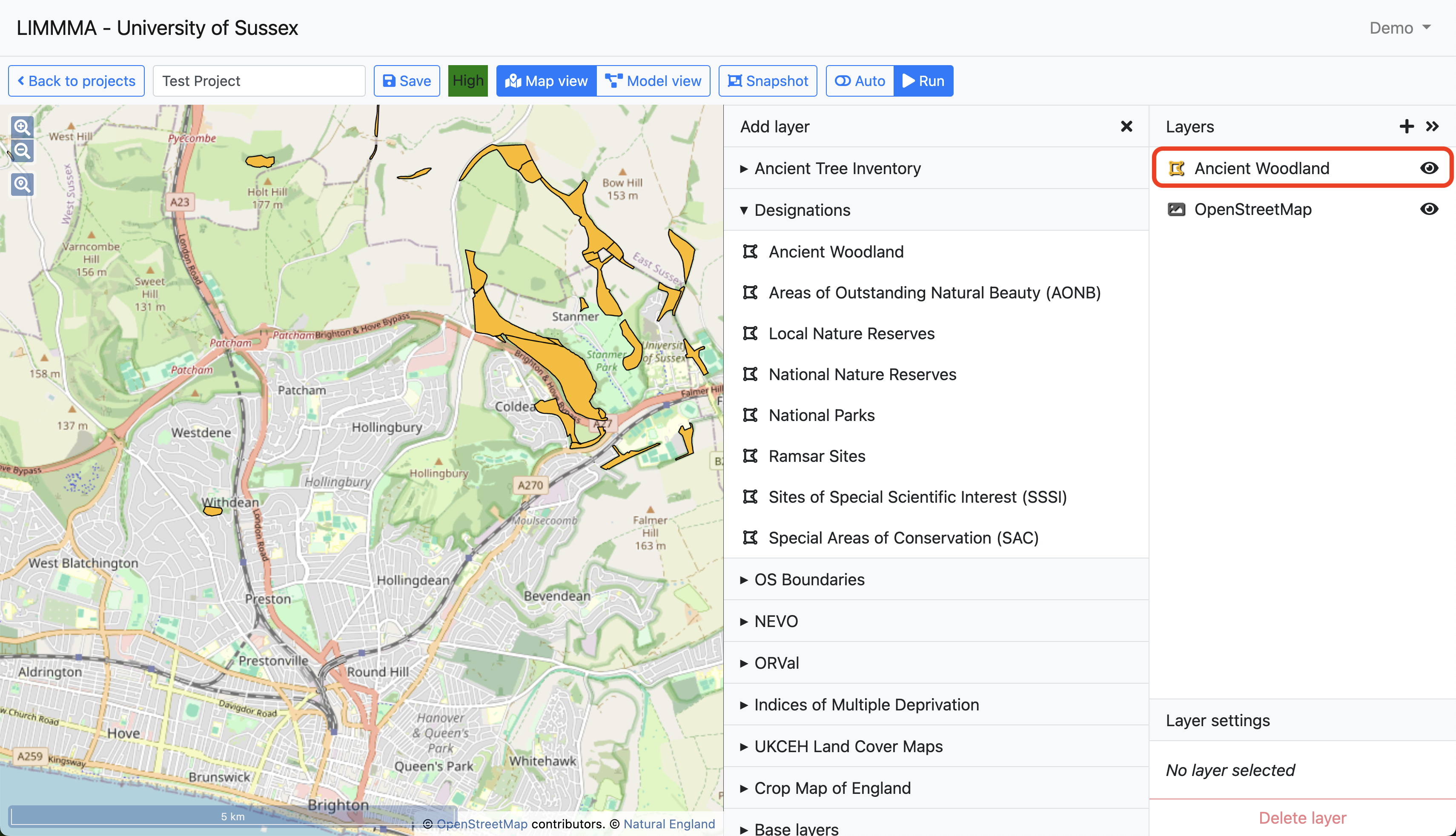
This is the most straightforward way of adding a new map layer to examine alongside other layers in Map view. It also preserves the original layer’s data type (e.g. point data, vector data, raster data etc.). However, if you want to be able to use a map layer in analysis or to view statistics about a map layer it needs to be added in Model view which converts it to a format usable for modelling and generating statistics.

2.4 Model View

To enter the project Model view, click the button on the top menu bar labelled “Model view.” It will take you to the following screen.

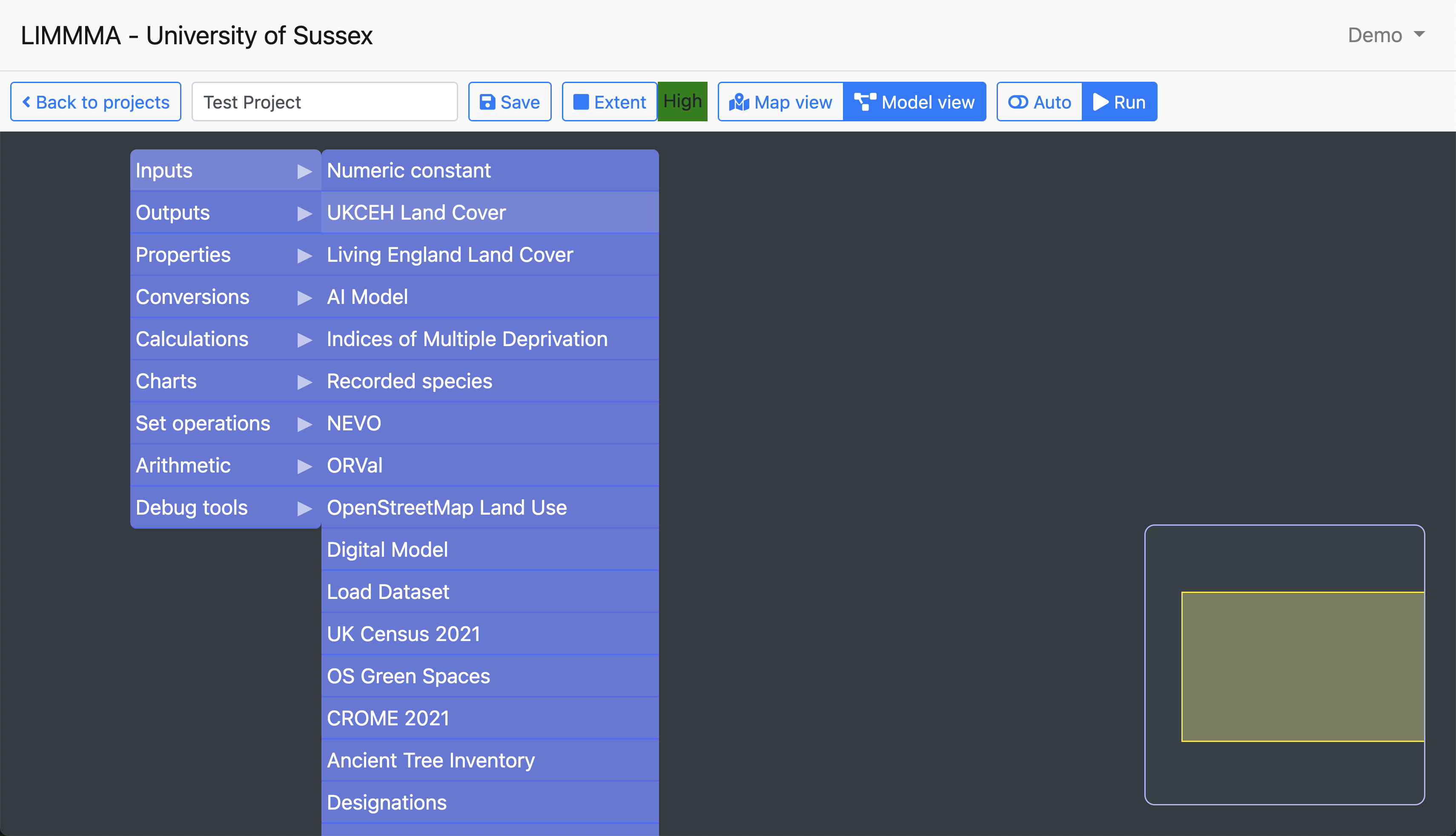
Right click the blank canvas to open the menu of model components.

You will see a list of component types to choose from including:

1. Inputs: import data into the model.
2. Outputs: add an output as a new layer in Map view or save it to your workspace datasets.
3. Properties: add area and unit properties to map layer output.
4. Conversions: convert data from number to numeric grid, numeric grid to number, boolean to categorical dataset.
5. Calculations: calculate area, create a distance map, return the cell area, or generate an interpolation from input data.
6. Charts: create a bar chart.
7. Set operations: perform set operations on boolean datasets.
8. Arithmetic: masking, expressions, and a set of simple mathematical functions to transform numerical datasets.

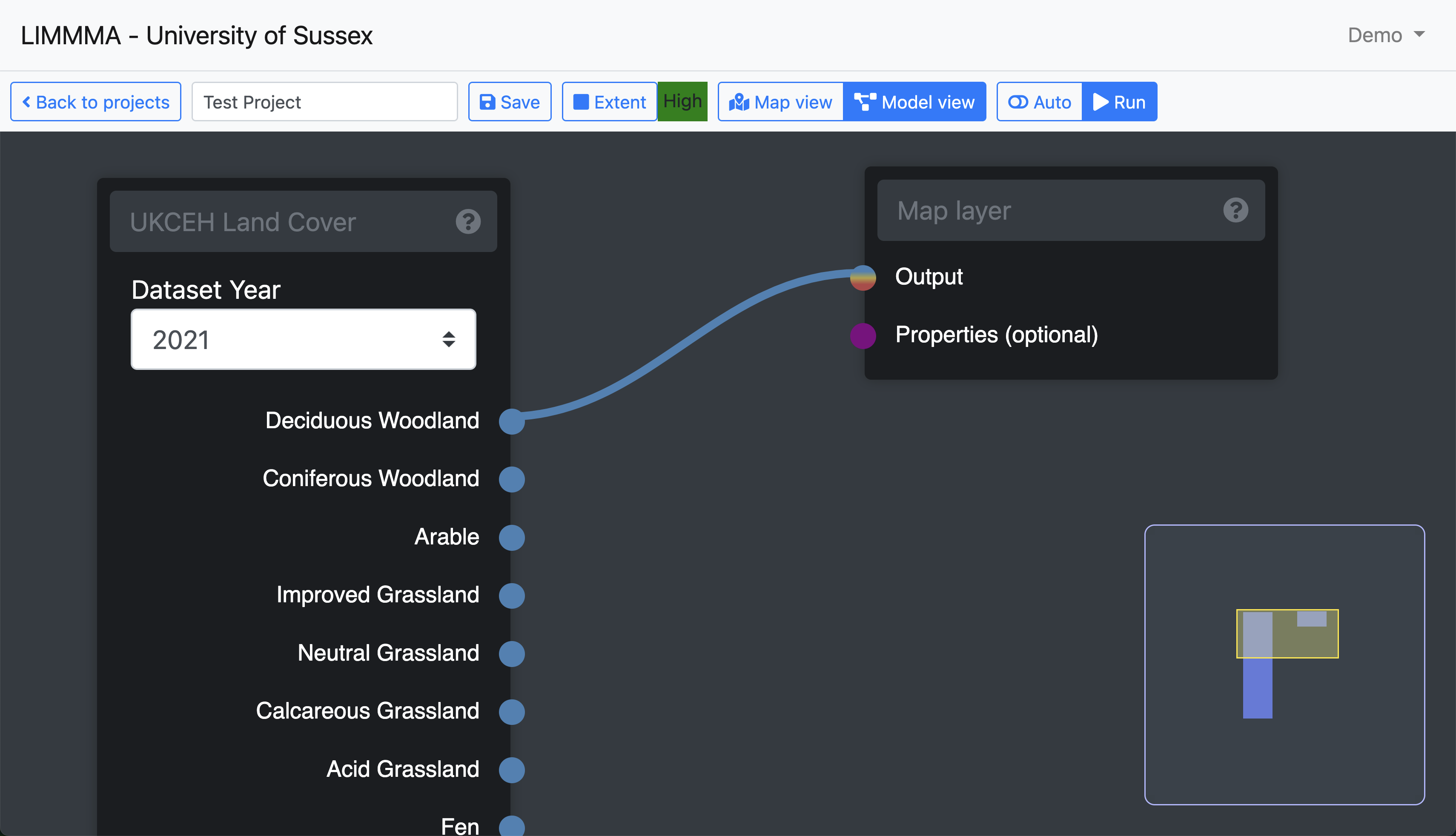
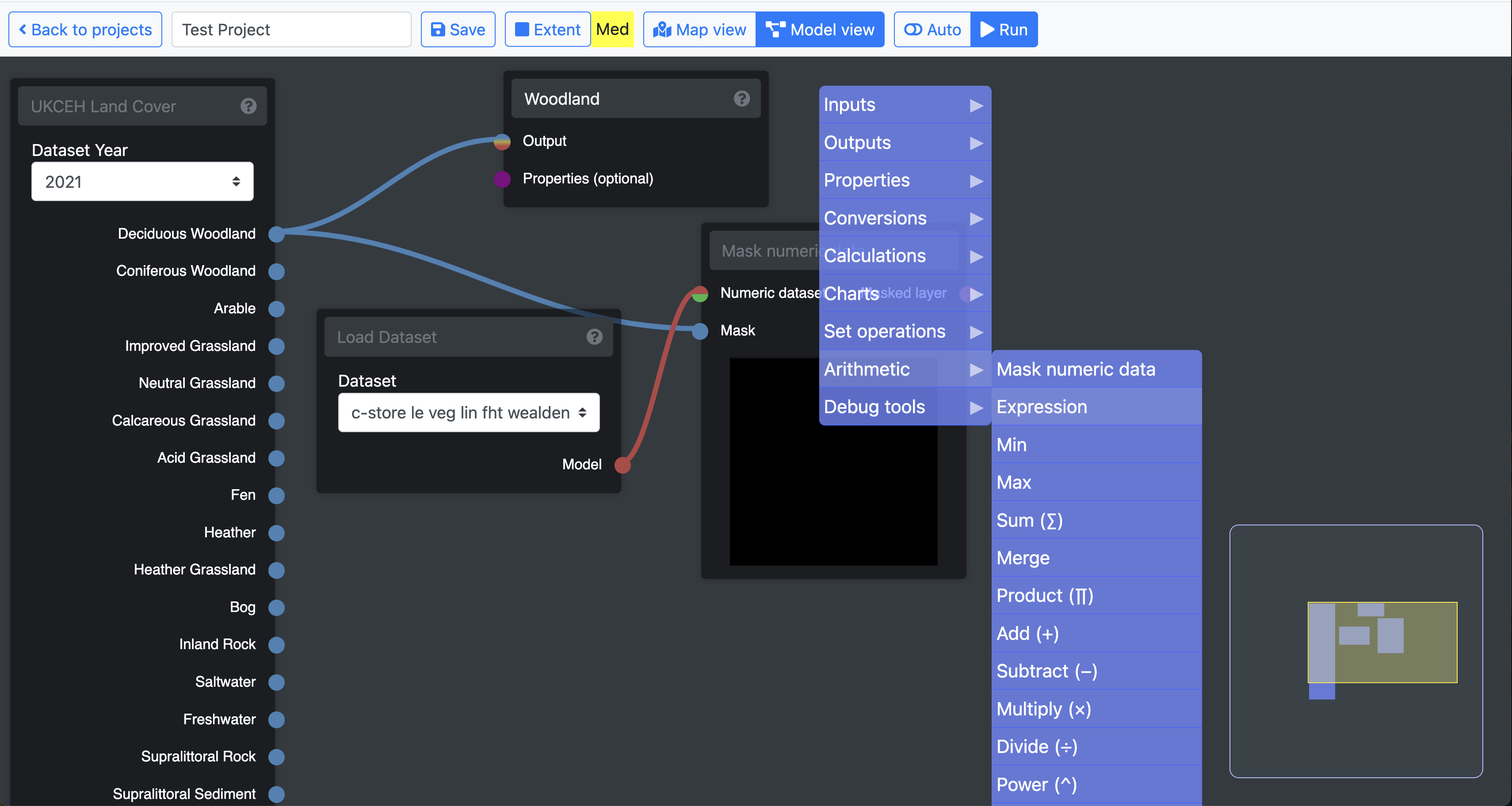
Hover the mouse over each category to see the list of components. Let’s chose UKCEH Land Cover from the Inputs category.

When you click the UKCEH Land Cover option it will add the component to the canvas from where you can interact with it (see below). It shows a box with a drop list to select the year and a set of blue nodes labelled for each type of land cover. These are the component’s output nodes because they appear on the right hand side. This component has no input nodes (which would appear on the left).

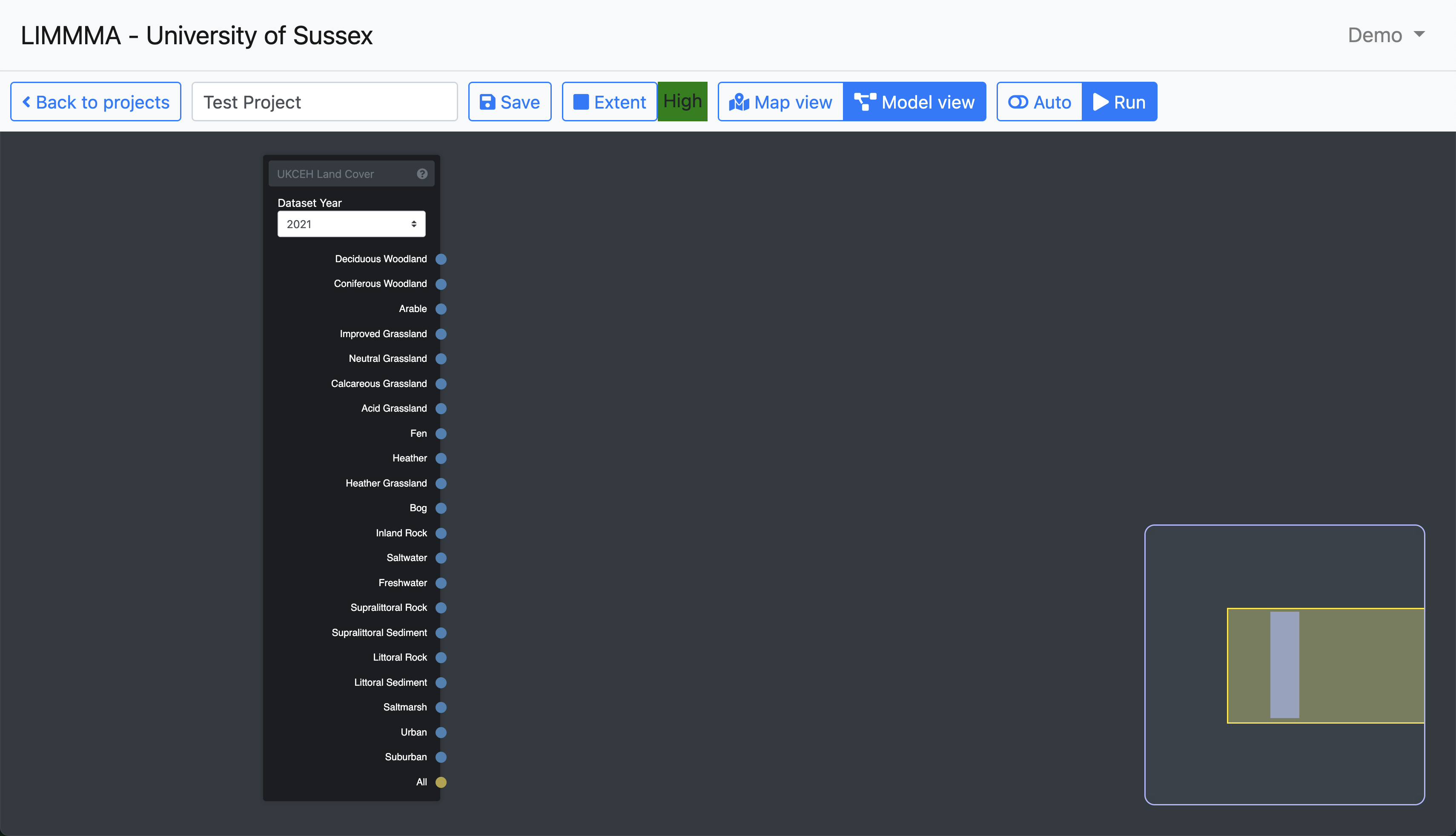
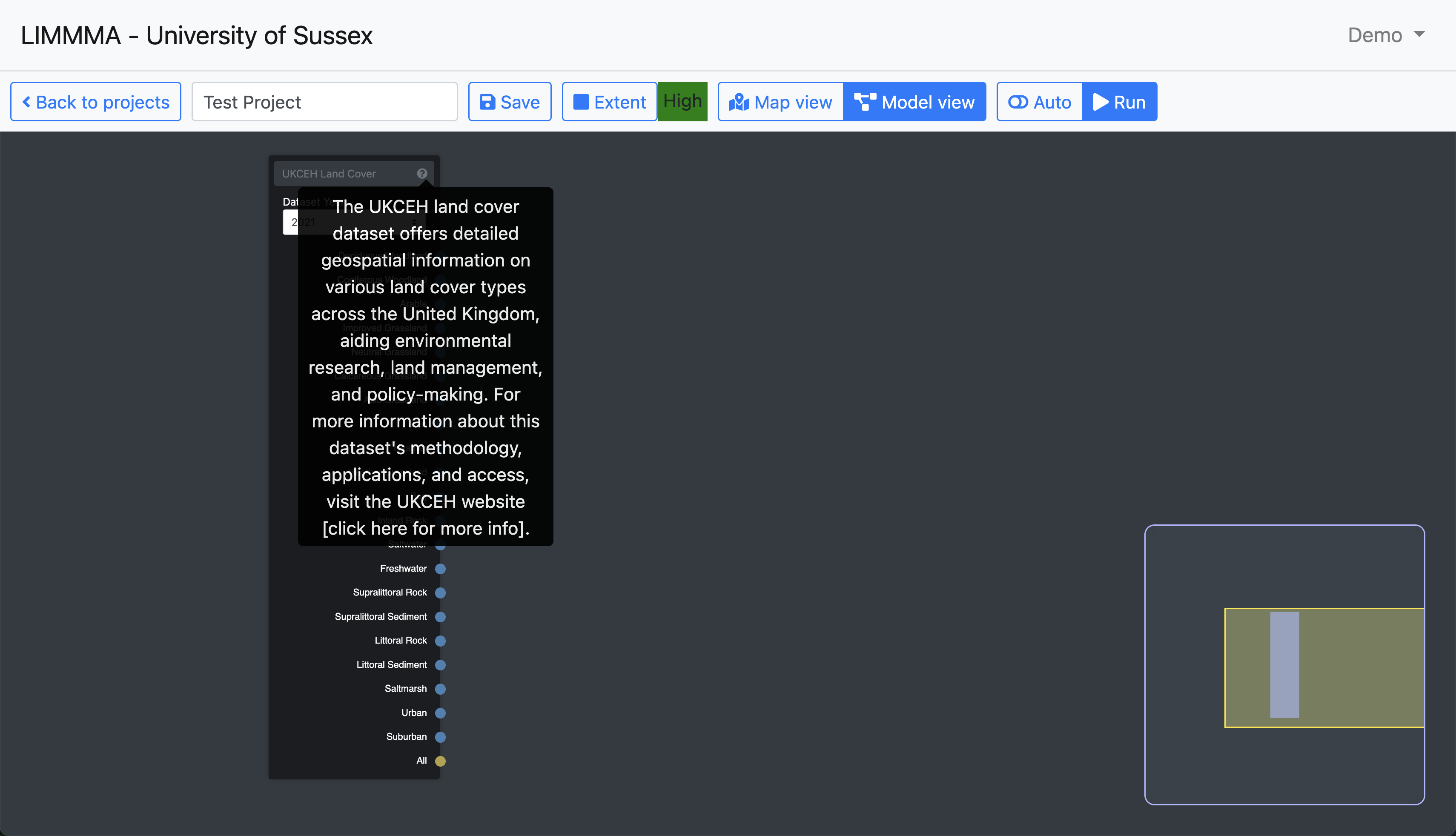
Hover the mouse over the “?” at the top right of the UKCEH component to see information about the dataset.

Now let’s say we want to create a new map layer showing only “Deciduous Woodland” from the UKCEH dataset. We can do this using the “Output” component called “Map layer”.

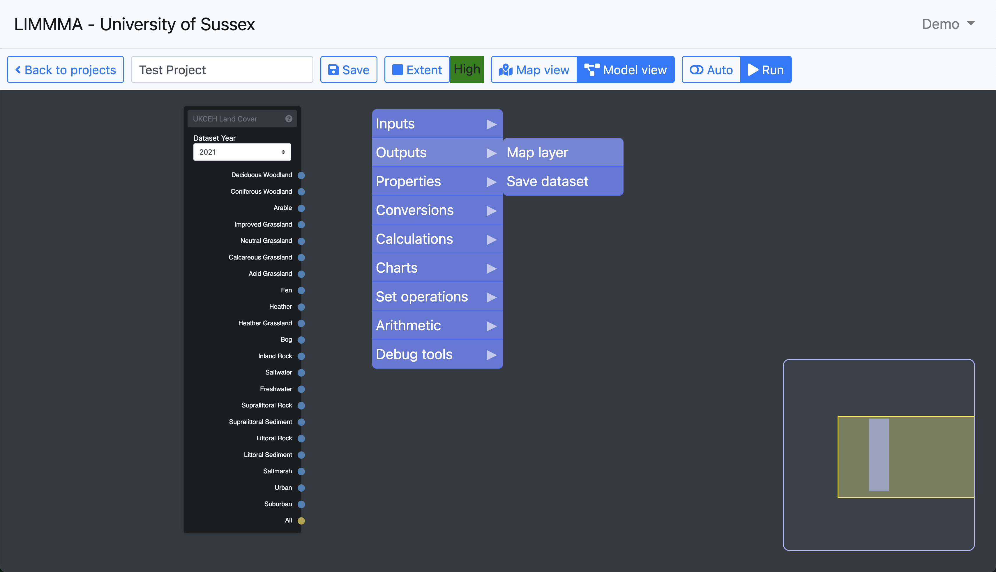
The “Map layer” component takes two inputs indicated by the nodes on its left hand edge. The top input node is labelled “Output” because it determines what is sent as an output to Map view. The “Properties” input takes area and unit properties which are used to label the map layer in Map view. These are optional so we will ignore them for now.

Make sure the year 2021 is selected on the UKCEH component and then click and drag from the “Deciduous Woodland” node to the input node on the Map layer component labelled “Output” (see below). Rename the Map layer component to something like “Woodland”. This is the name that will appear in Map view as the label for the new map layer.

Now save and run the model. When the run process is complete you can switch back to Map view by clicking the button on the top menu bar.

It is difficult to see the new Woodland layer because the default colours are white for TRUE and transparent for FALSE (i.e. areas of woodland show up as white while areas which are not woodland are invisible). As the new layer is overlaid on top of the OpenStreetMap layer the white areas of woodland are barely visible. Let’s see how to manipulate map layers to make them more visible and meaningful as we view them overlaid on one another.

2.5 Manipulating map layers

The layer colour options can be viewed by clicking the layer and opening the “Layer legend.”

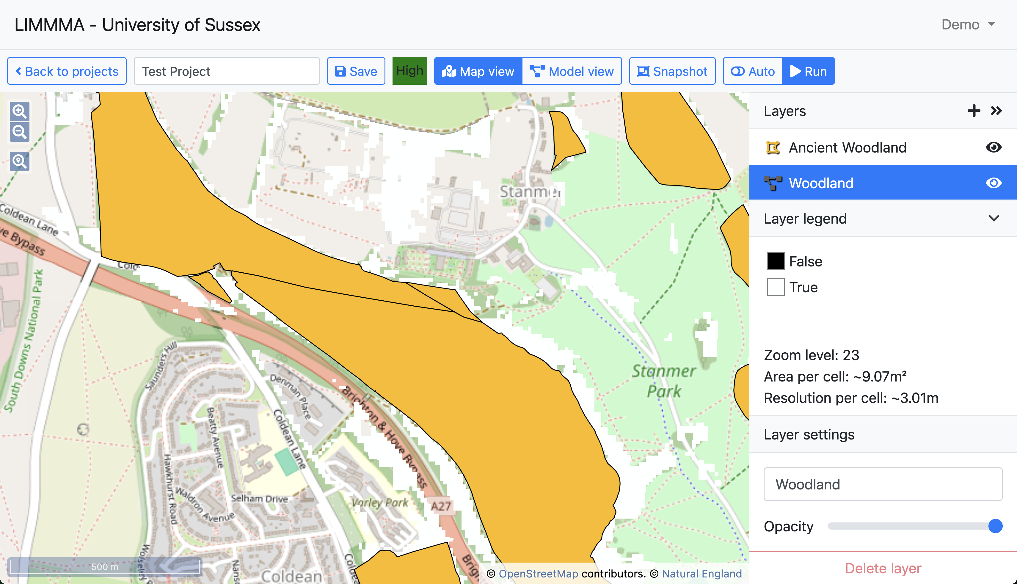
Click the white square next to the label TRUE and select a colour from the colour palette.

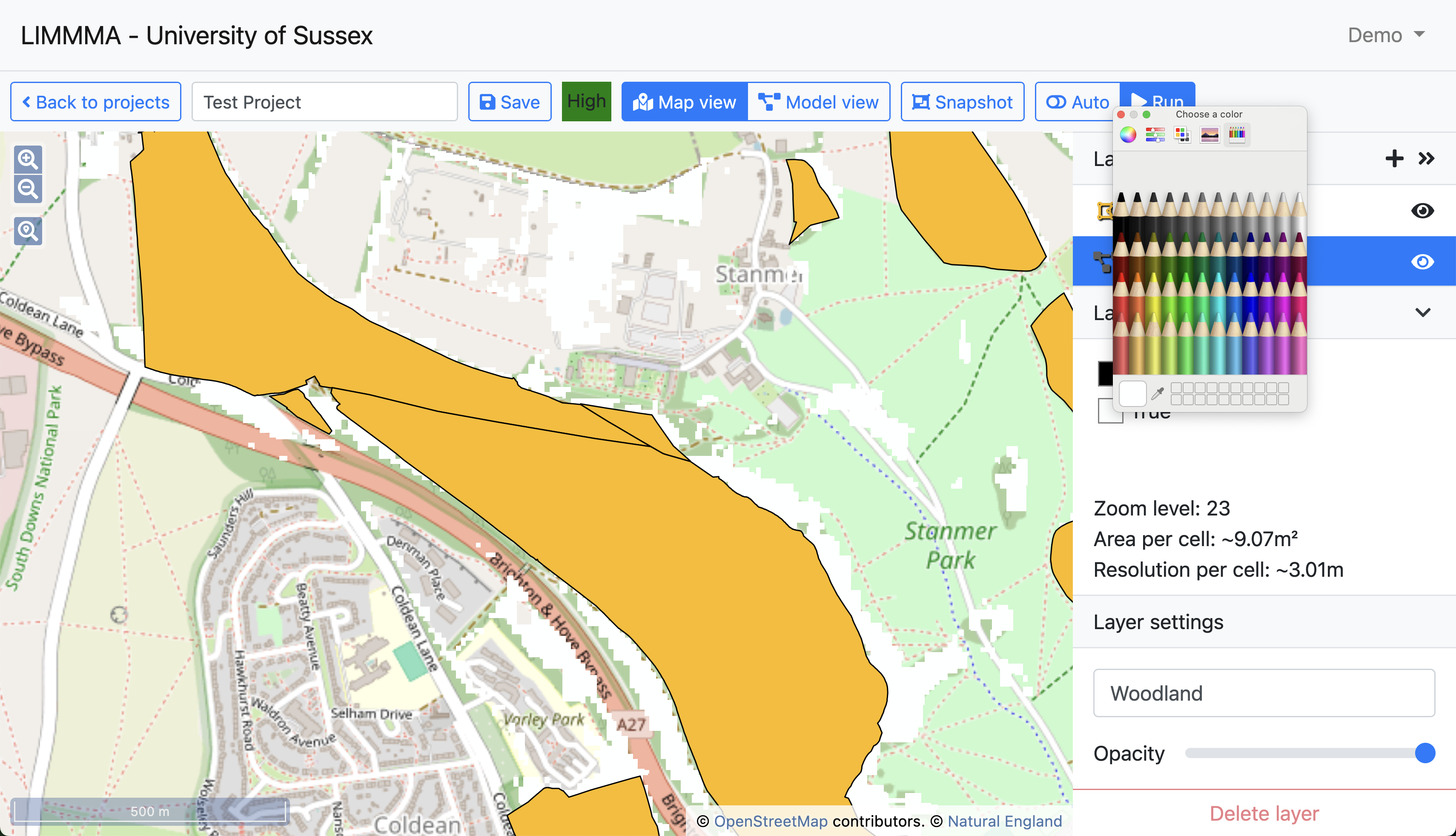
Now you will see the colour on the map change to match your selection.

Tip

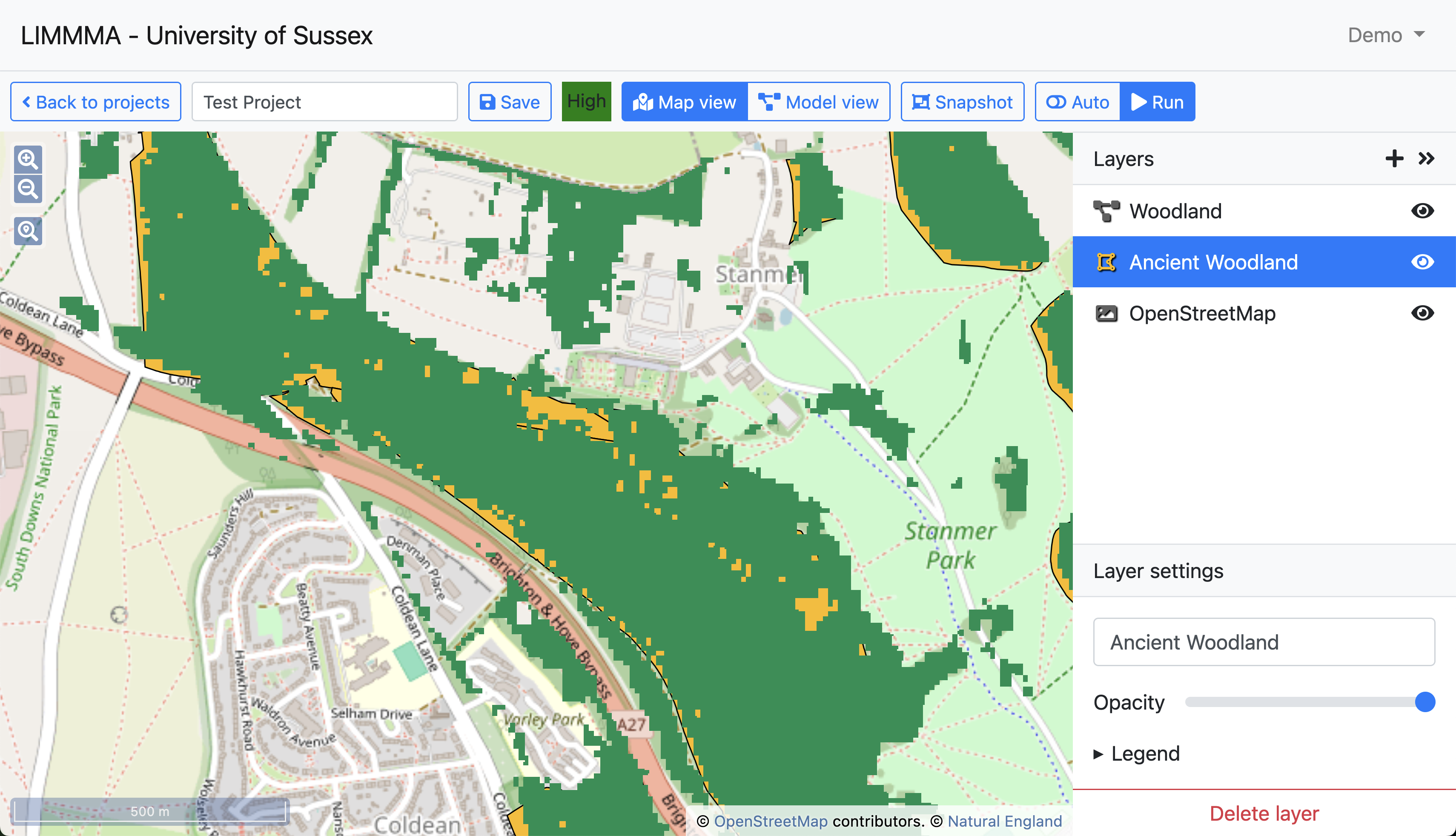
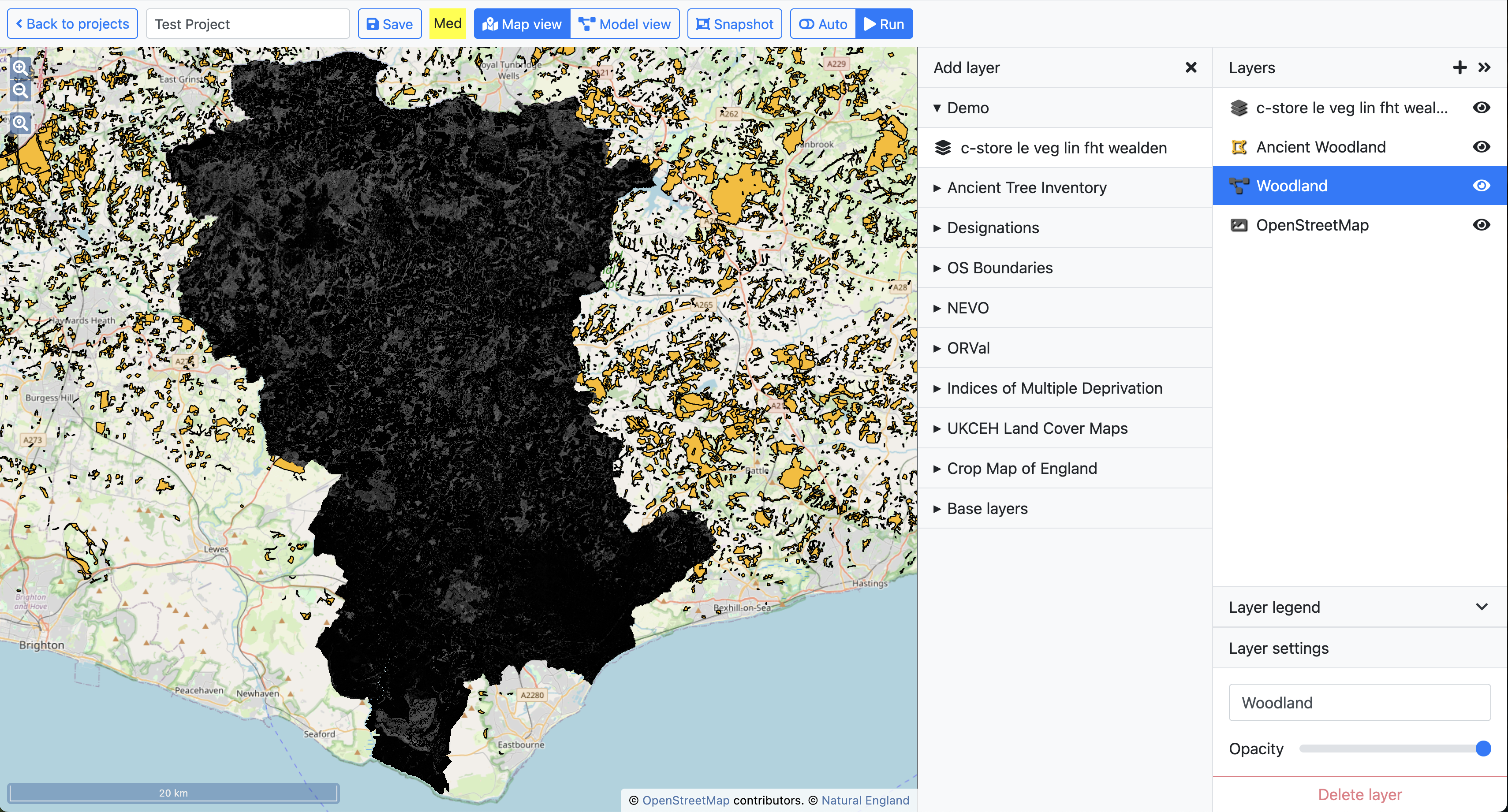
You will notice that the “Woodland” layer is displayed as small grid squares. This is because the original data has been converted into a raster format (i.e. grid squares) to match the project resolution and zoom level - in this case zoom level 23 with a cell resolution of around 3x3m.

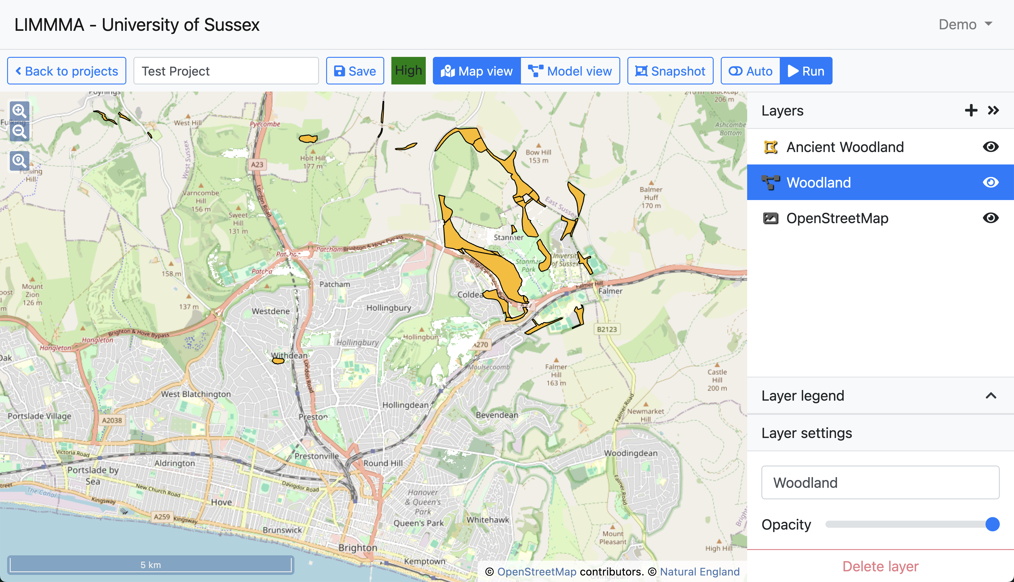
Map layers can be re-ordered by clicking and dragging each layer up and down in the right hand sidebar. Each layer in the sidebar is displayed over all the layers below it. Click on the Woodland layer and drag it to the top of the stack of layers to see how the map view changes.

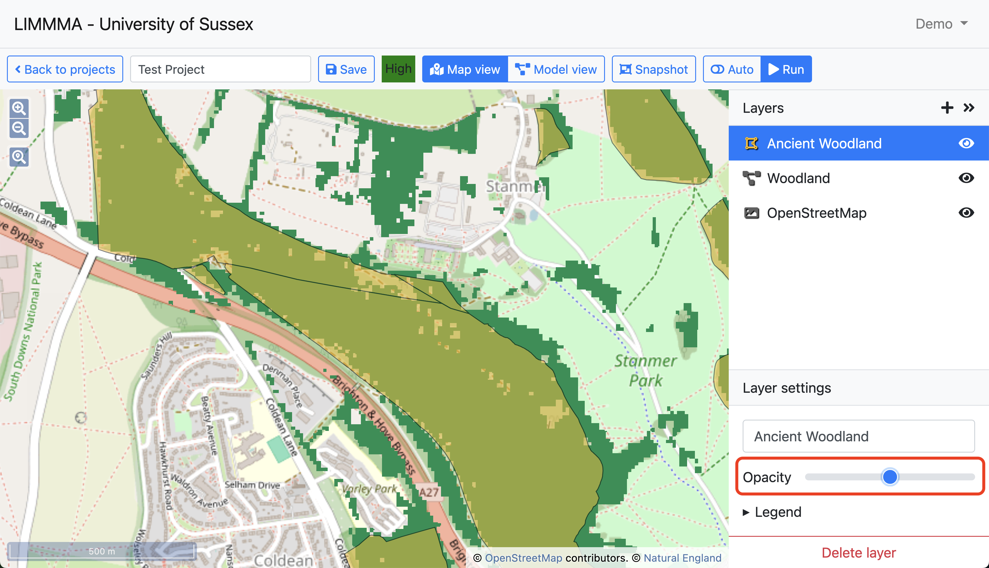
The opacity of each layer can be adjusted to allow you to view one or more layers simultaneously. Now let’s put the Woodland layer back where it was, directly below the Ancient Woodland layer. Next, click on the Ancient Woodland layer, open “Layer settings” and adjust the opacity slider until you begin to see the new Woodland layer below. Now we can clearly see to what extent the designated areas of Ancient Woodland overlap with the extent of Deciduous Woodland recorded in 2021.

As mentioned above, adding a new map layer in this way (via the Model view) means you can view information about it directly in Map view and via the Snapshot tool.

2.6 Layer information

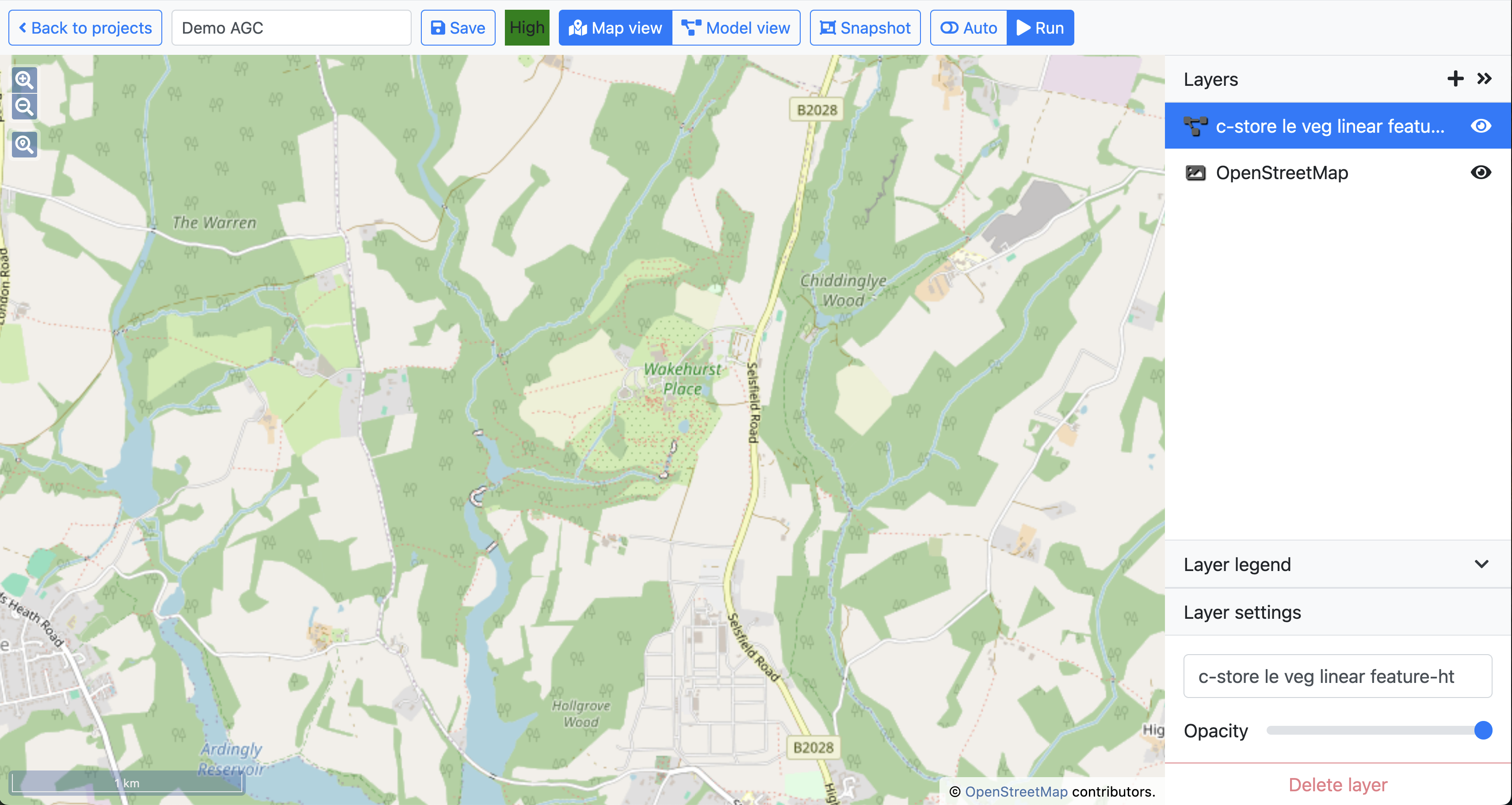
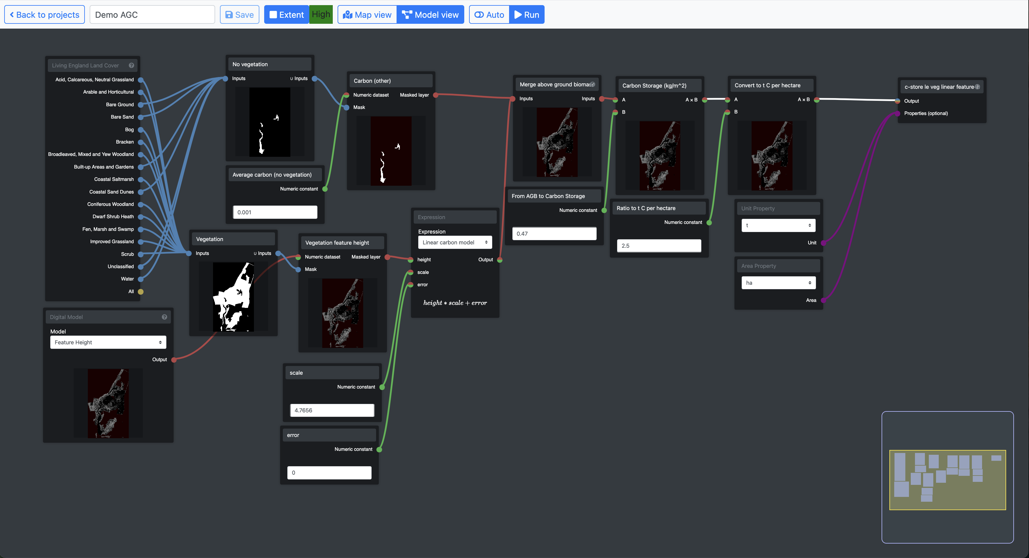
After saving the current project, return to the project menu and open the demonstration project called “Demo AGC.” This has been set up for you with a model to estimate above ground carbon in the landscape of Kew Wakehurst using a habitat basemap and lidar data measuring feature height for all habitats containing vegetation. Feel free to toggle Model view to see how the model is structured.

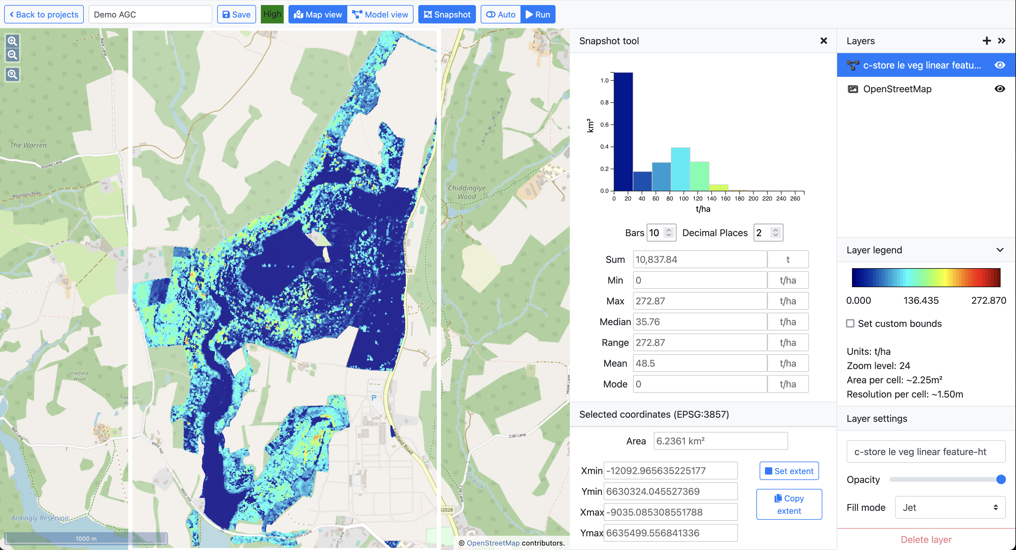
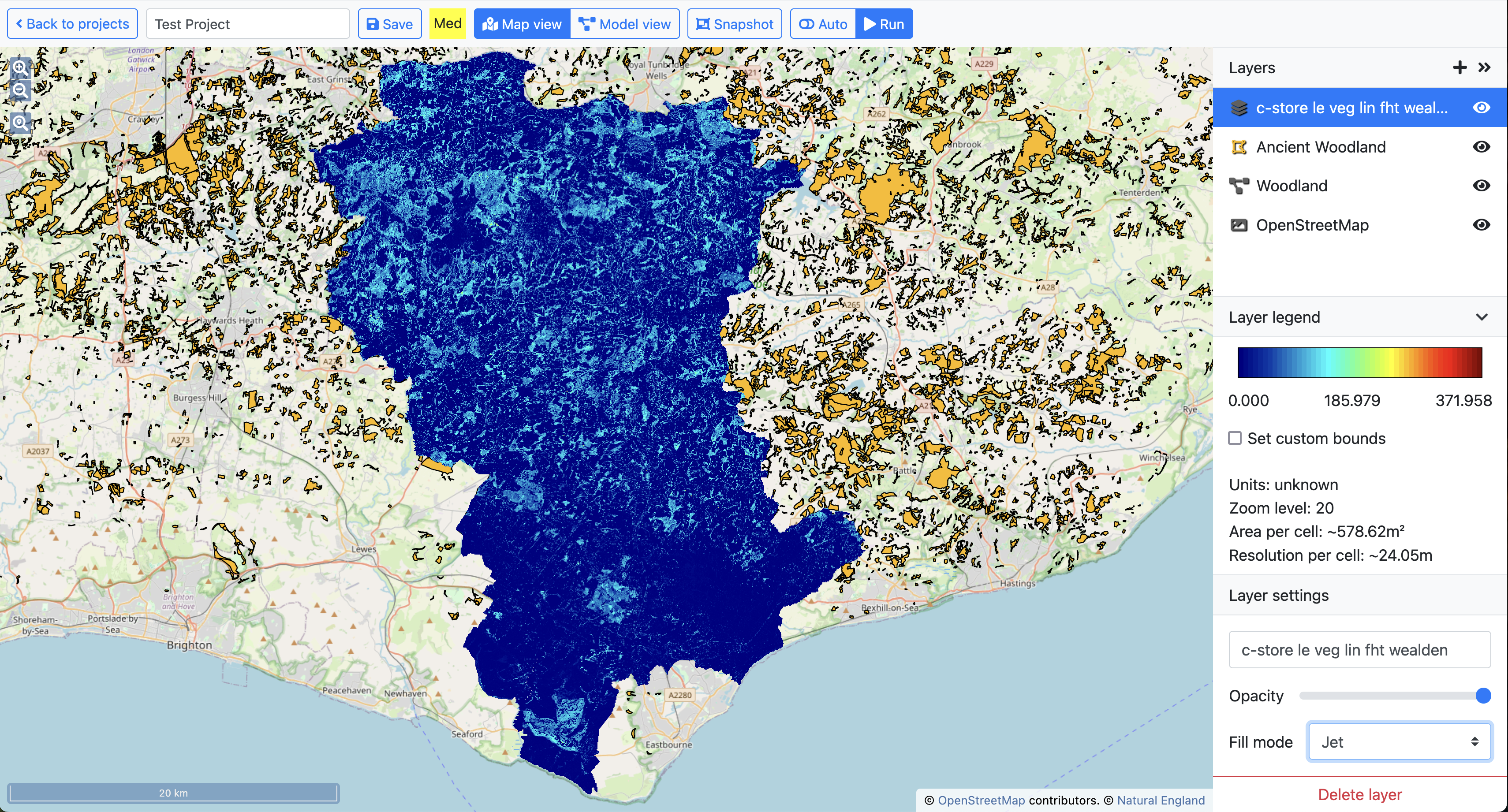
In Map view you will notice a map layer called “c-store le veg linear feature-ht”. It won’t show any data until you run the model.

Click “Run” and wait a moment for the model to create the map layer. It should look like this:

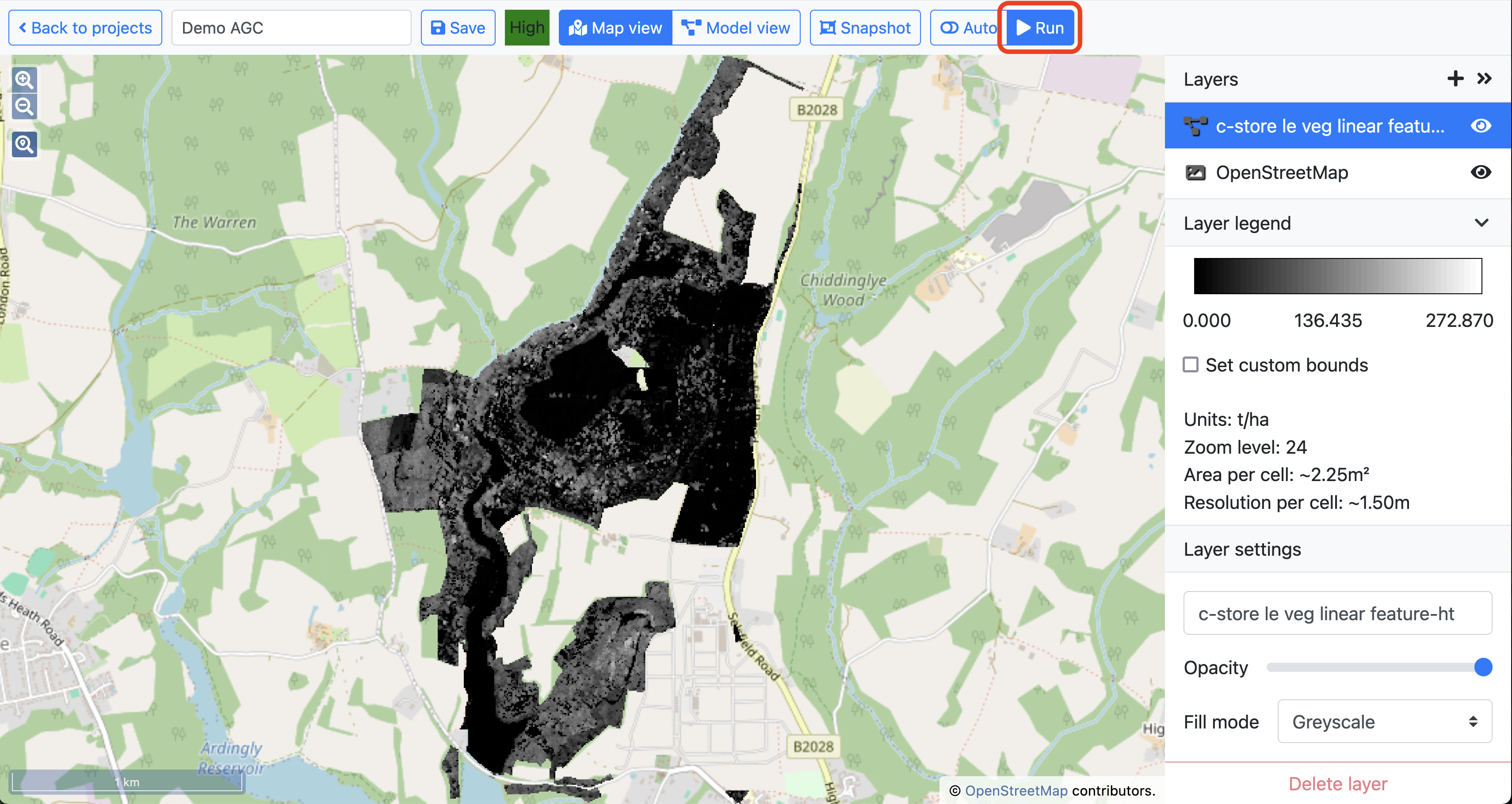
Notice that the “Layer legend” now shoes a gradient bar of values from 0 to 272.87 with units of t/ha. The model has generated a raster layer representing organic carbon density. The density in t/ha of organic carbon estimated for each cell (1.5x1.5m) is represented as shade of grey from black (minimum) to white (maximum).

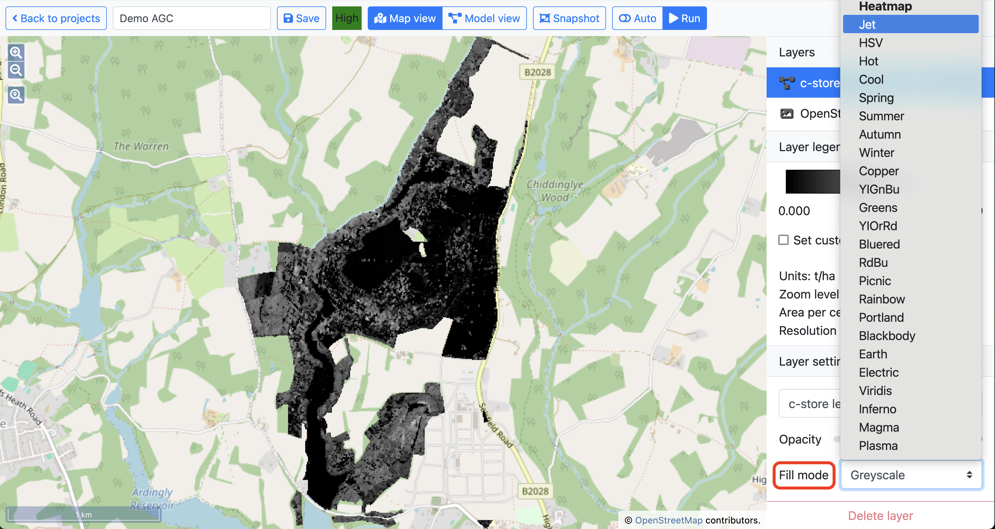
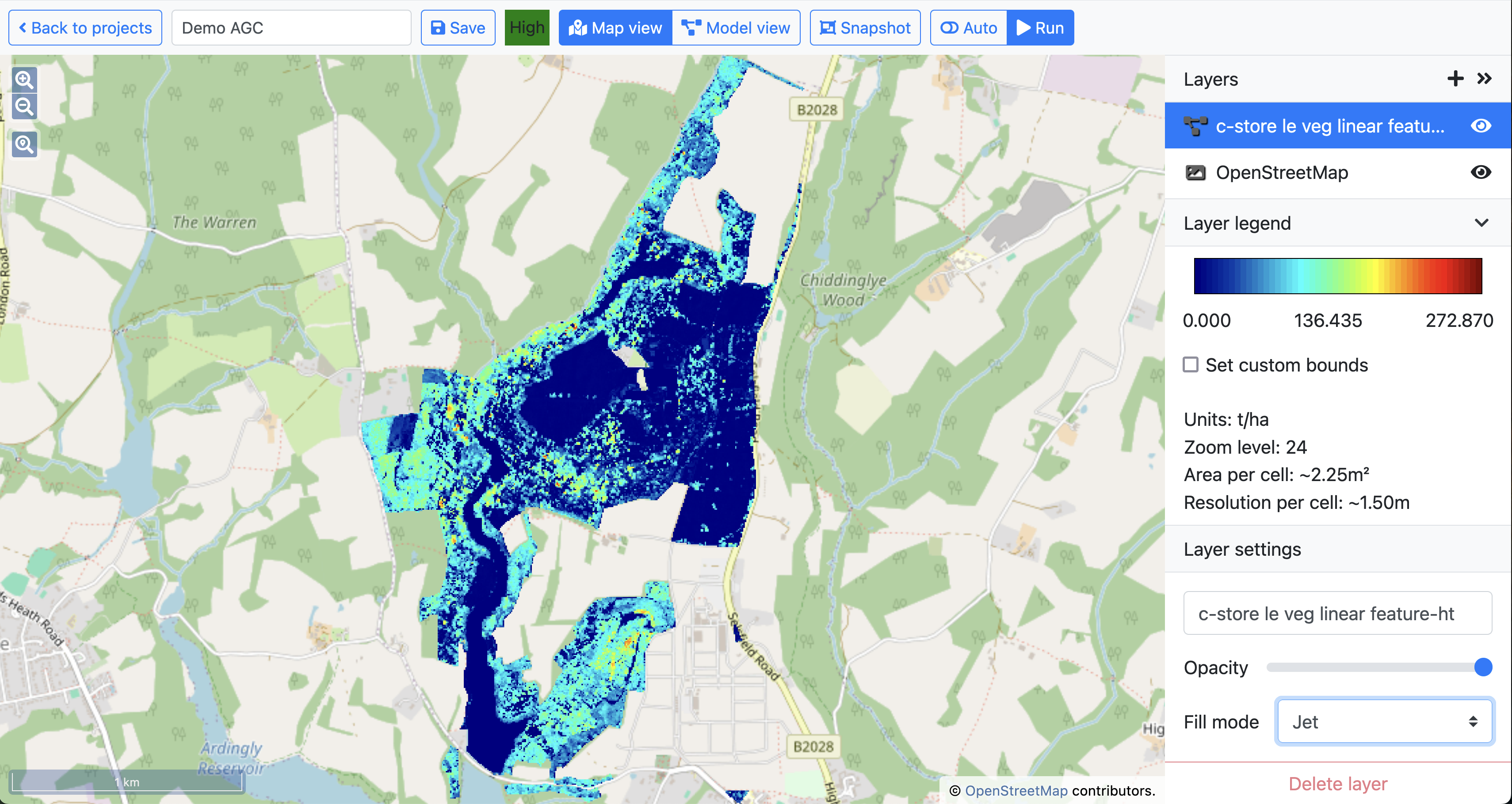
To change the colour of the gradient go to the “Layer settings” and click on “Fill mode”. From the drop down list you can select whatever fill mode you want. Let’s try “Jet.”

The map is much easier to read with this adjustment.

Now let’s take a look at some more detailed information about the c-store layer.

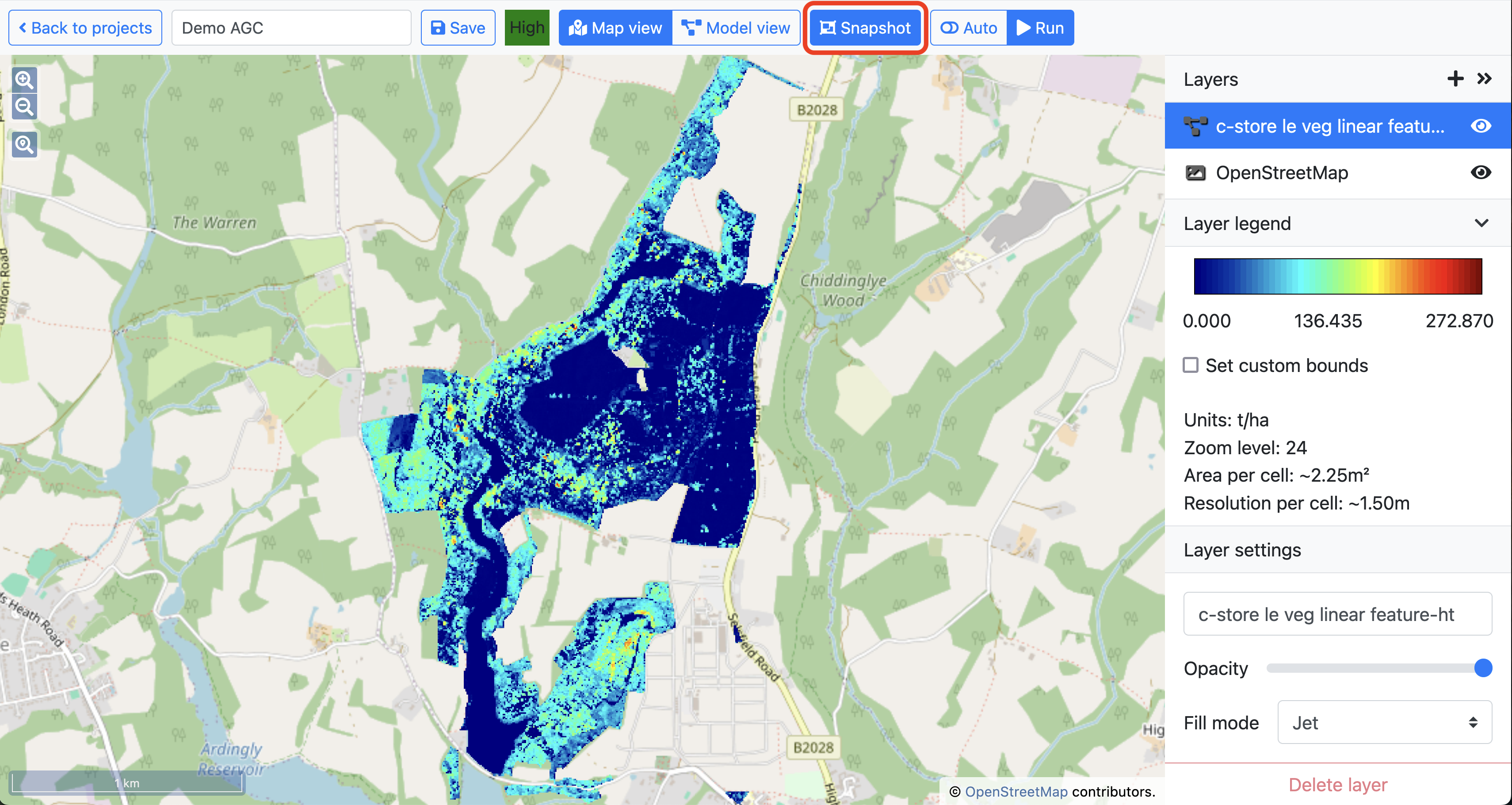
2.7 Snapshot tool

The Snapshot tool is used to view graphs and statistical information about a map layer. Click “Snapshot” on the top menu bar to open the tool.

The tool opens a new panel alongisde the layer menu and the map.

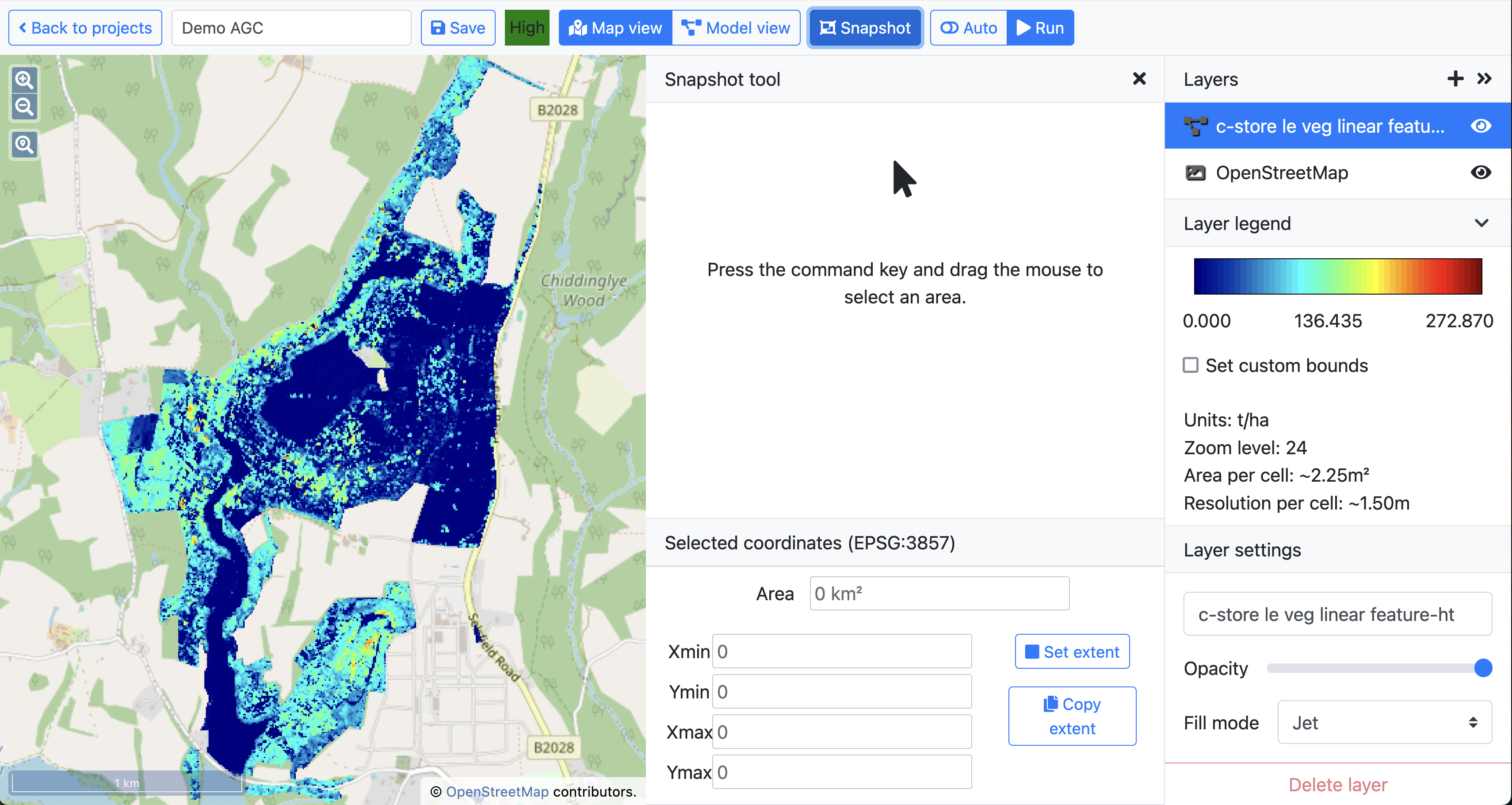
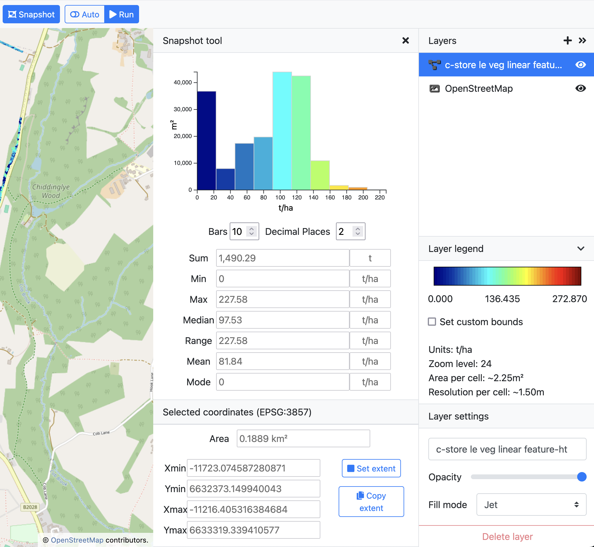
To select an area to snapshot, hold down the command key and click and drag the mouse on the map. The Snapshot tool will immediately display a graph and some summer statistics about the area of the layer which you have selected.

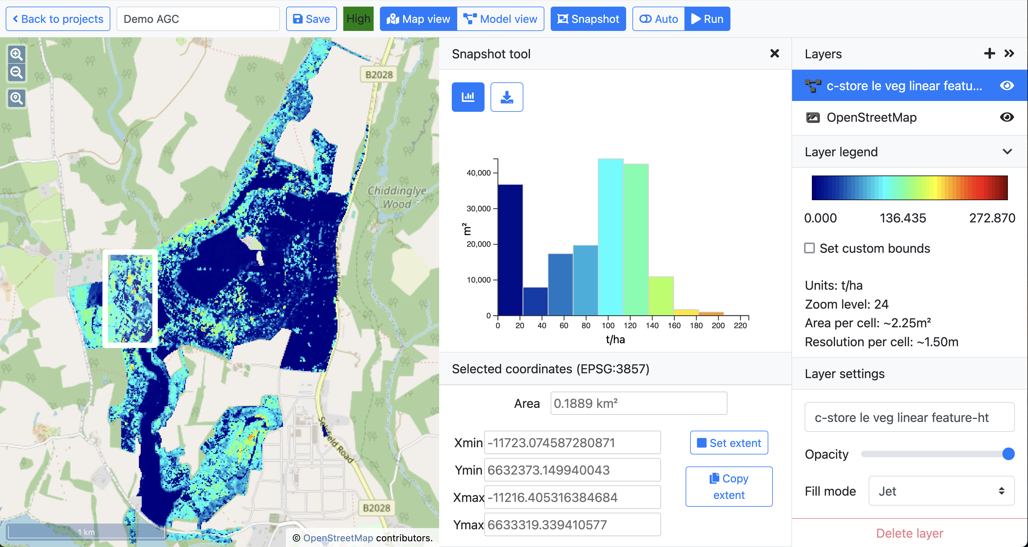
Below the graph, you should also see a list of values for Sum, Min, Max, Median, Range and Mean. In addition to adjusting the decimal places of these values you can also adjust the number of bars displayed in the graph above.

If you want to see a graph and stats for the whole project area you can simply click “Set extent” and then select “Use project extent.”

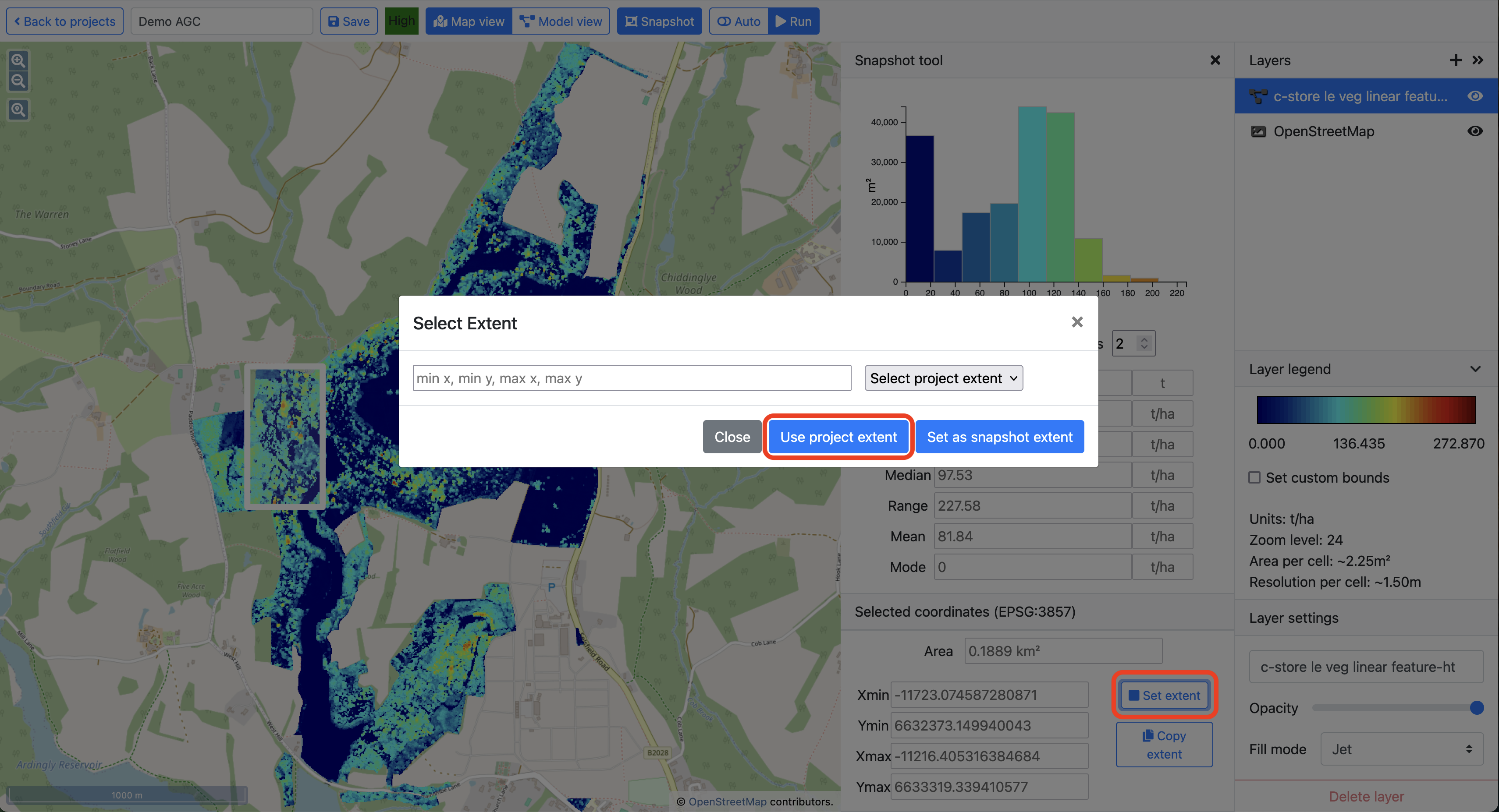
The tool will now show you the same information for the entire project extent (indicated within the white highlight box on the map).

2.8 Scaling

Now let’s say we want to run the same carbon model for a larger area such as the whole of the Wealden District Council. We can do this from Model view by clicking the “Extent” button on the top menu bar.

This takes you to the project extent page where you choose a new extent to run the model on.

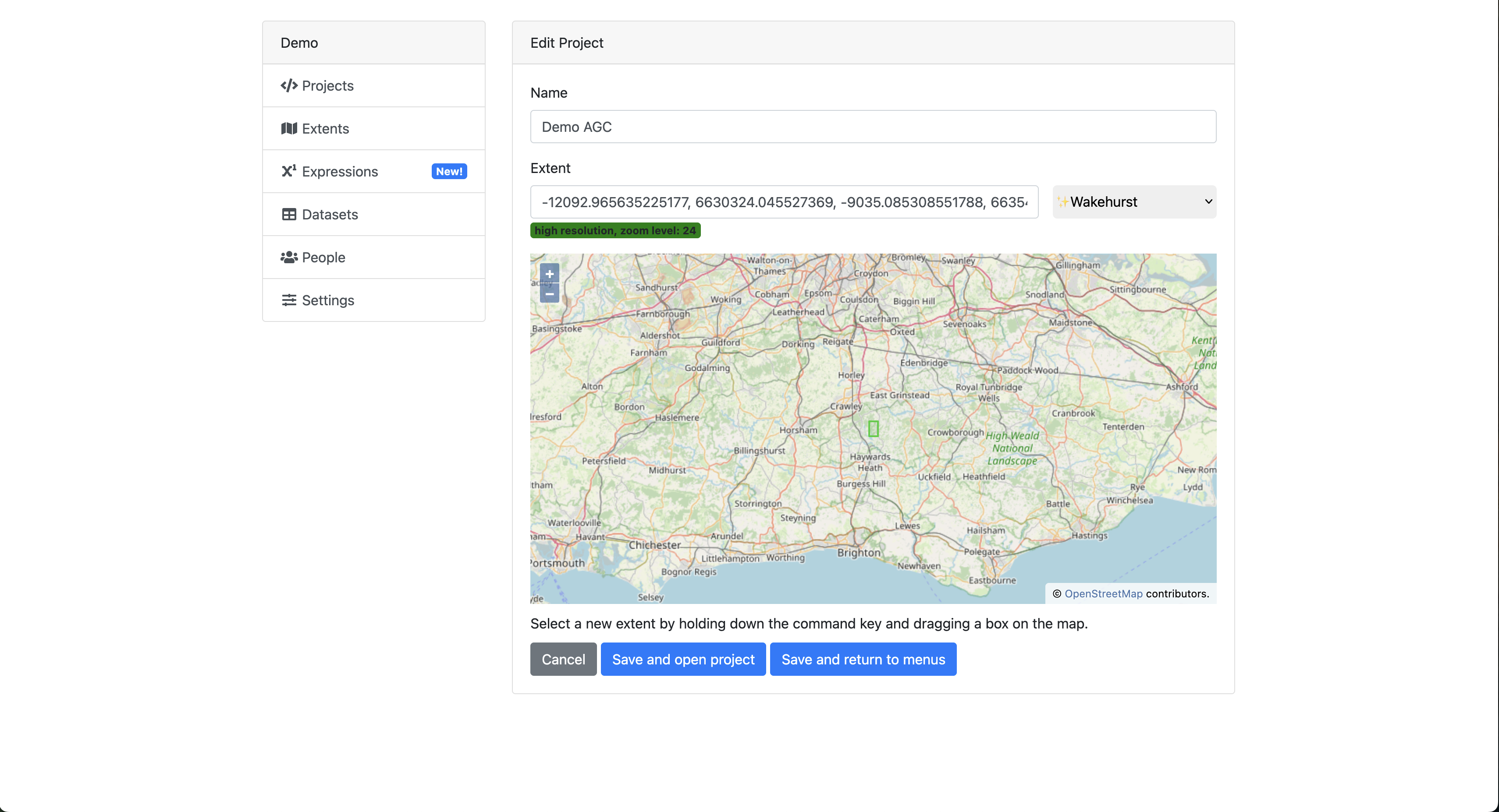
It is currently set to Wakehurst. Click the drop down and select “Wealden District Council.”

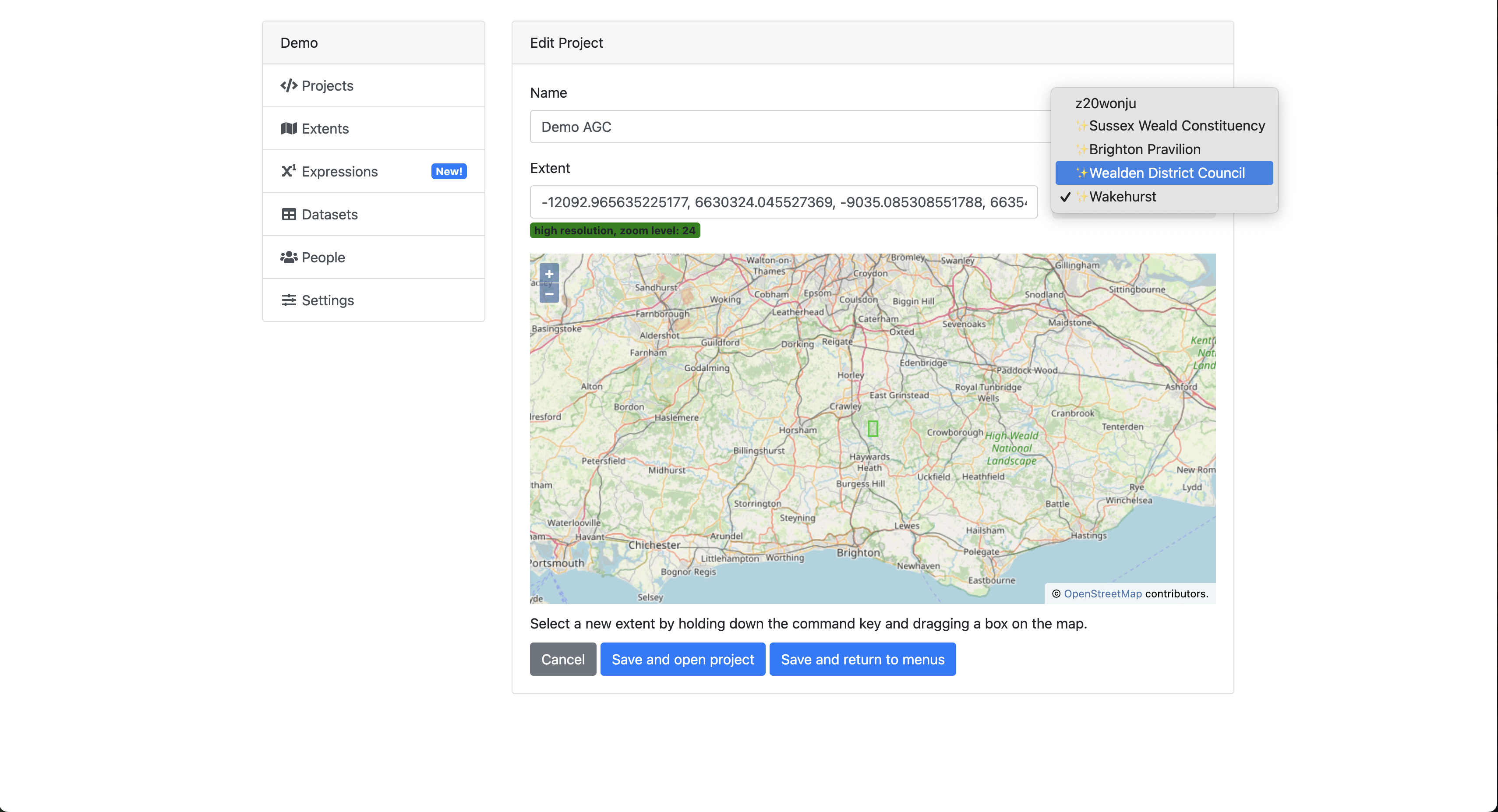
You will notice that the map shows the new extent and an updated zoom level of 20 since the area is much larger than the Wakehurst extent.

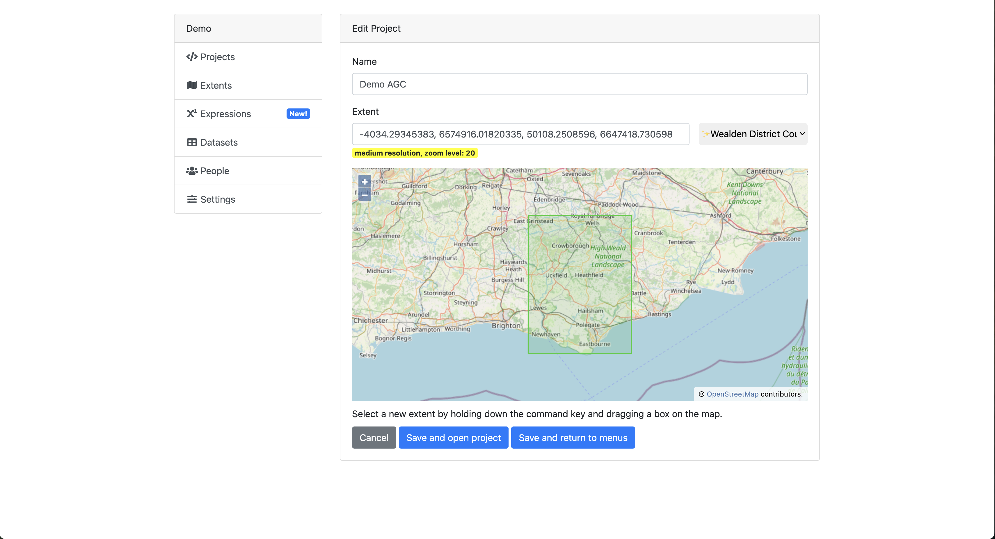
Click “Save and open project” and you will be taken back to the project Map view. If you hover the mouse over the yellow “Med” box on the top menu bar and it will display the extent on the map.

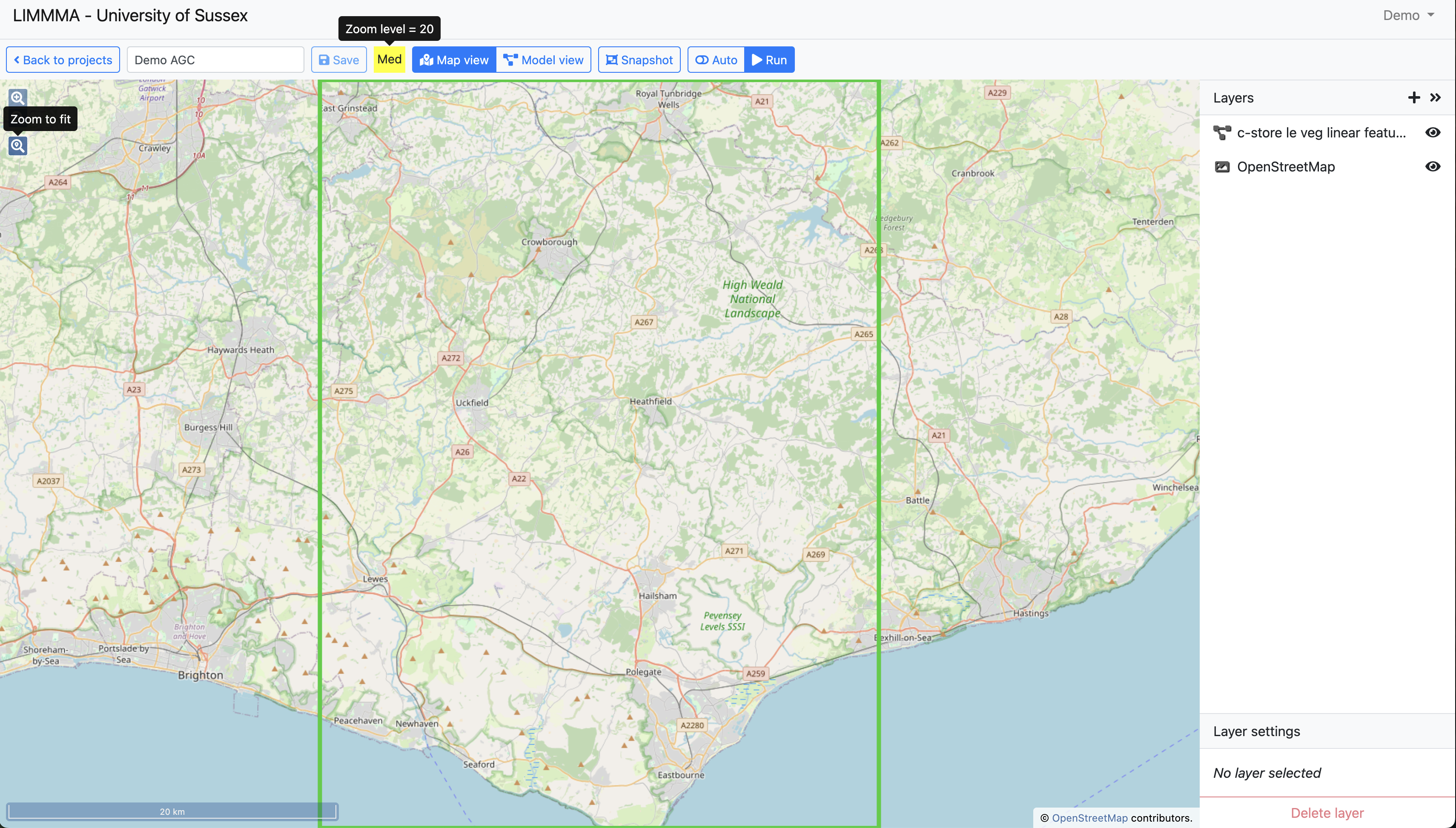
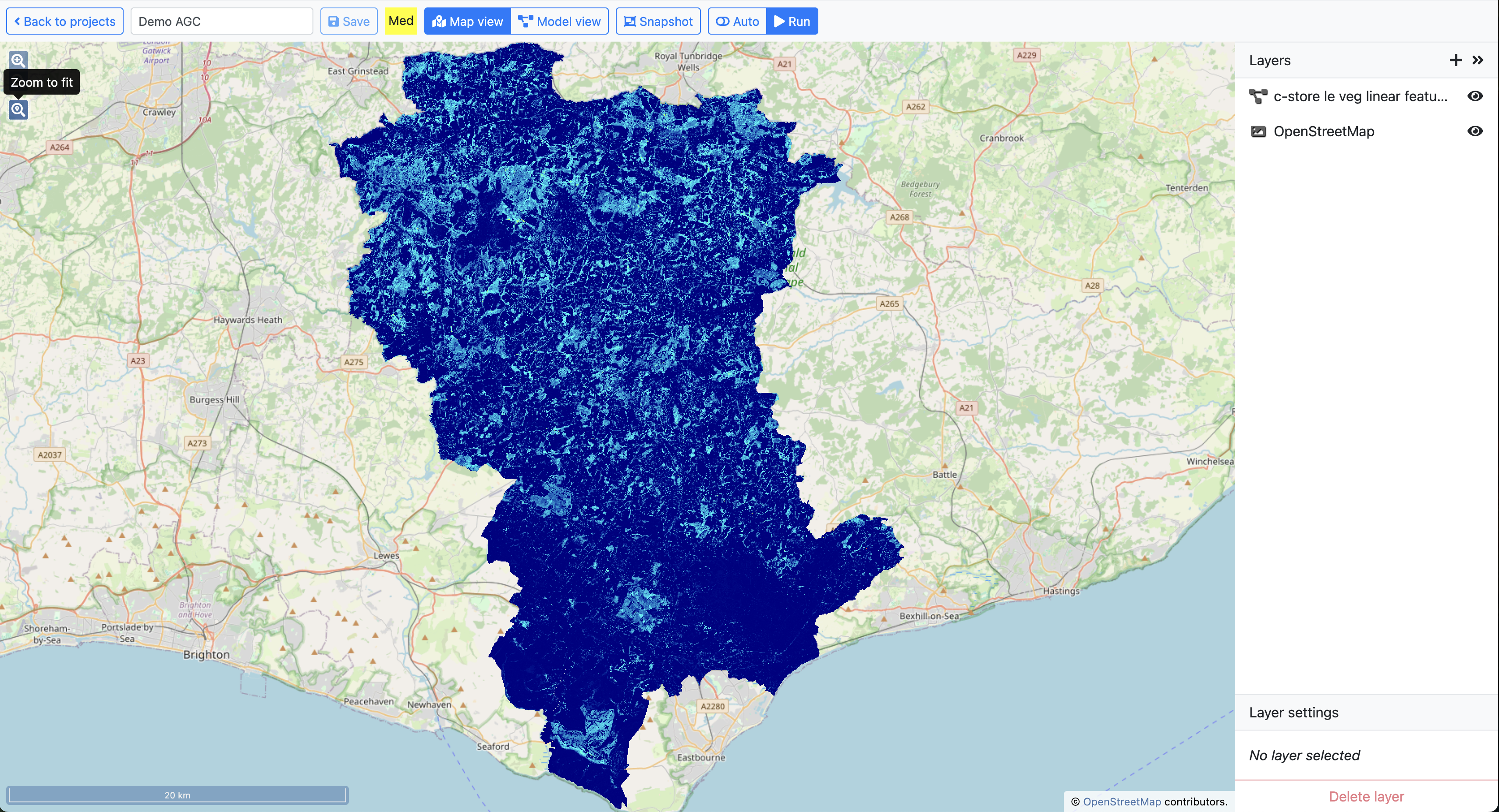
Now click “Run” and wait while the model is processing. After a few seconds the c-store layer will be updated as a map covering the Wealden District Council area.

2.9 Saving datasets

Now we might want to save this c-store layer as a dataset to use in other projects. For example we could create a new project to compare the results of this model with another model of stored organic carbon or combine it with a model of below soil carbon. Or perhaps we already have an opportunity map showing potential locations for nature recovery projects which we could use with the carbon map and other biodiversity data to explore the implications of implementing these projects across the landscape.

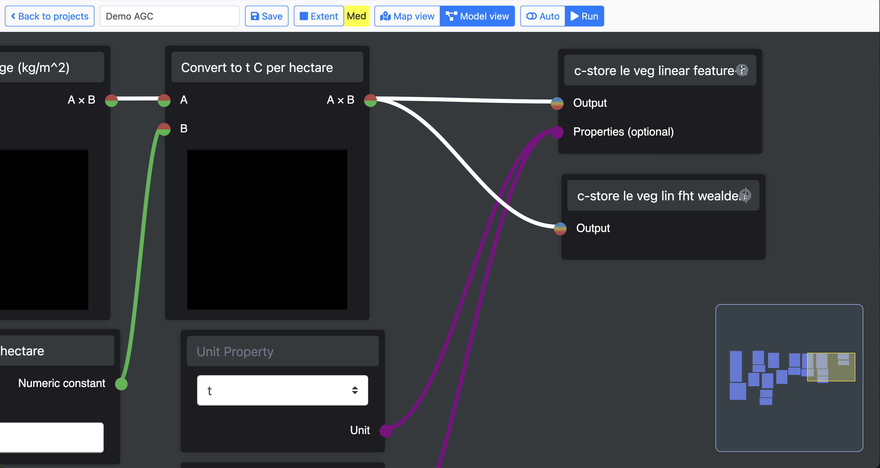
Back in Model view, right click the canvas and select from the Outputs list the component called “Save dataset.”

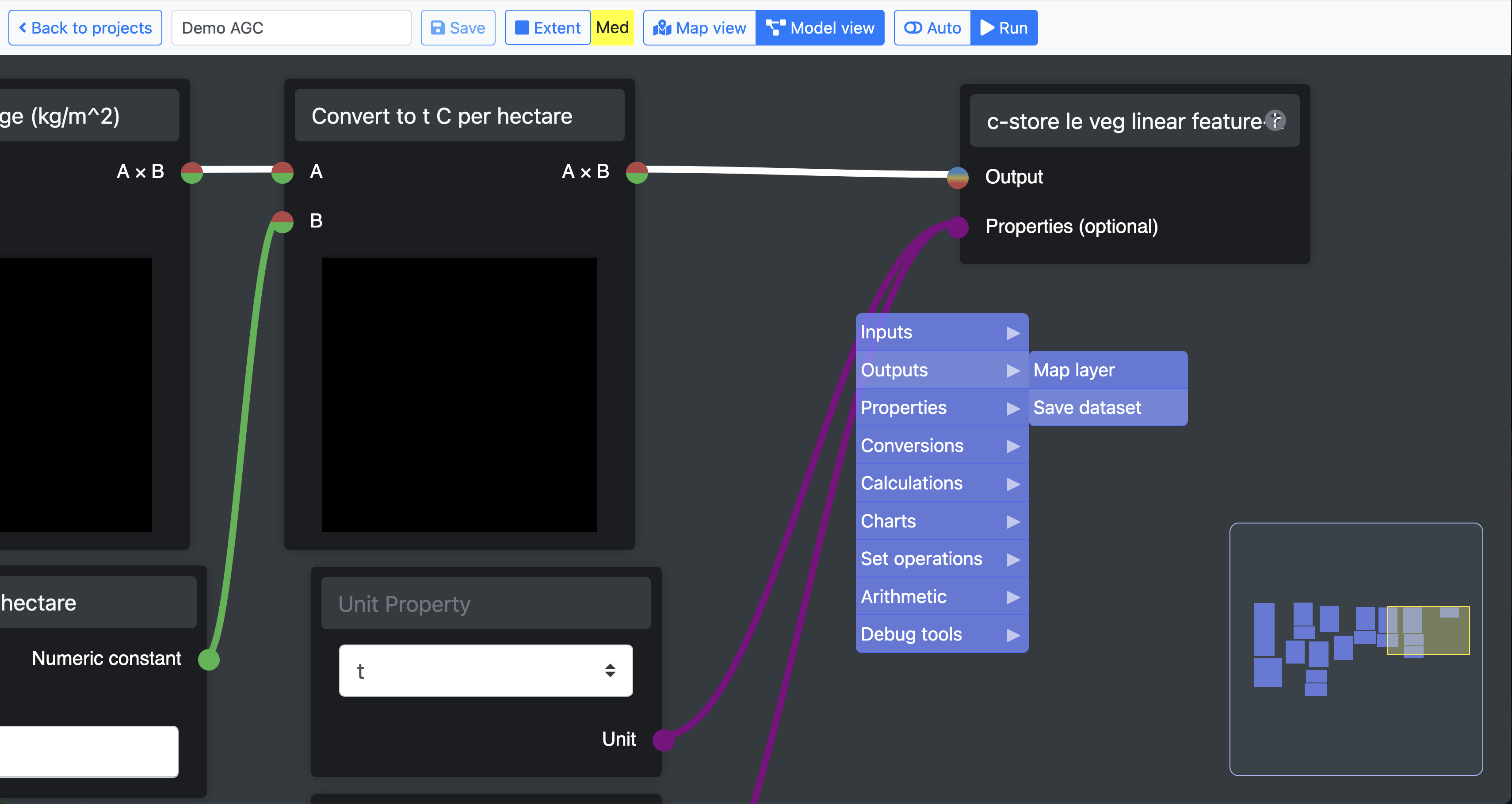
This component takes only one input to the node labelled “Output.”

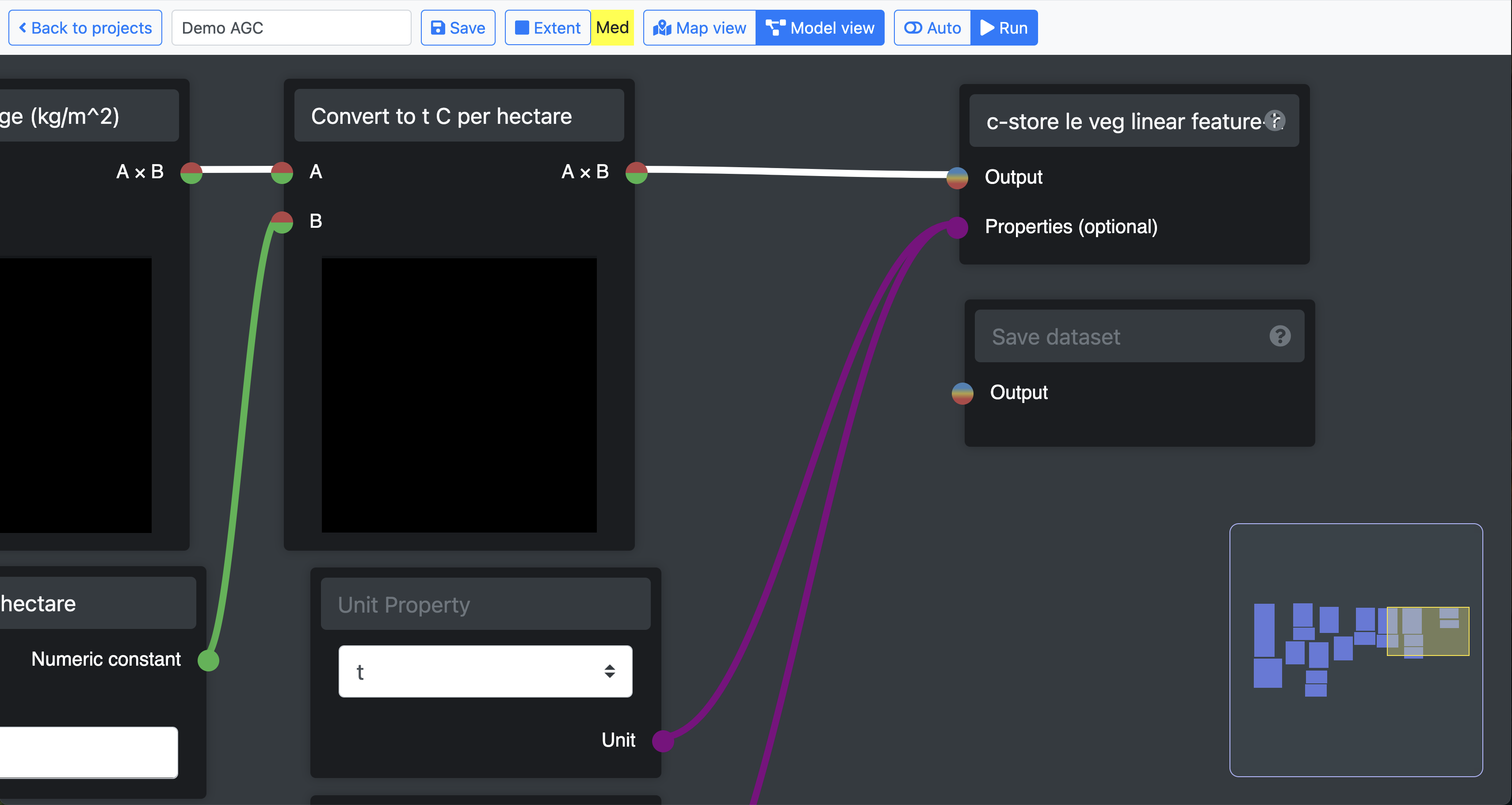
Connect the output from our model to the node on “Save datasets” and rename it something meaningful so you can find it again in the dataset menu. Then save the model and click “Run.” When the run process has completed the component will read “Saved!”

Now click “Back to projects” to return to the projects menu and click on “Datasets” to view your saved dataset.

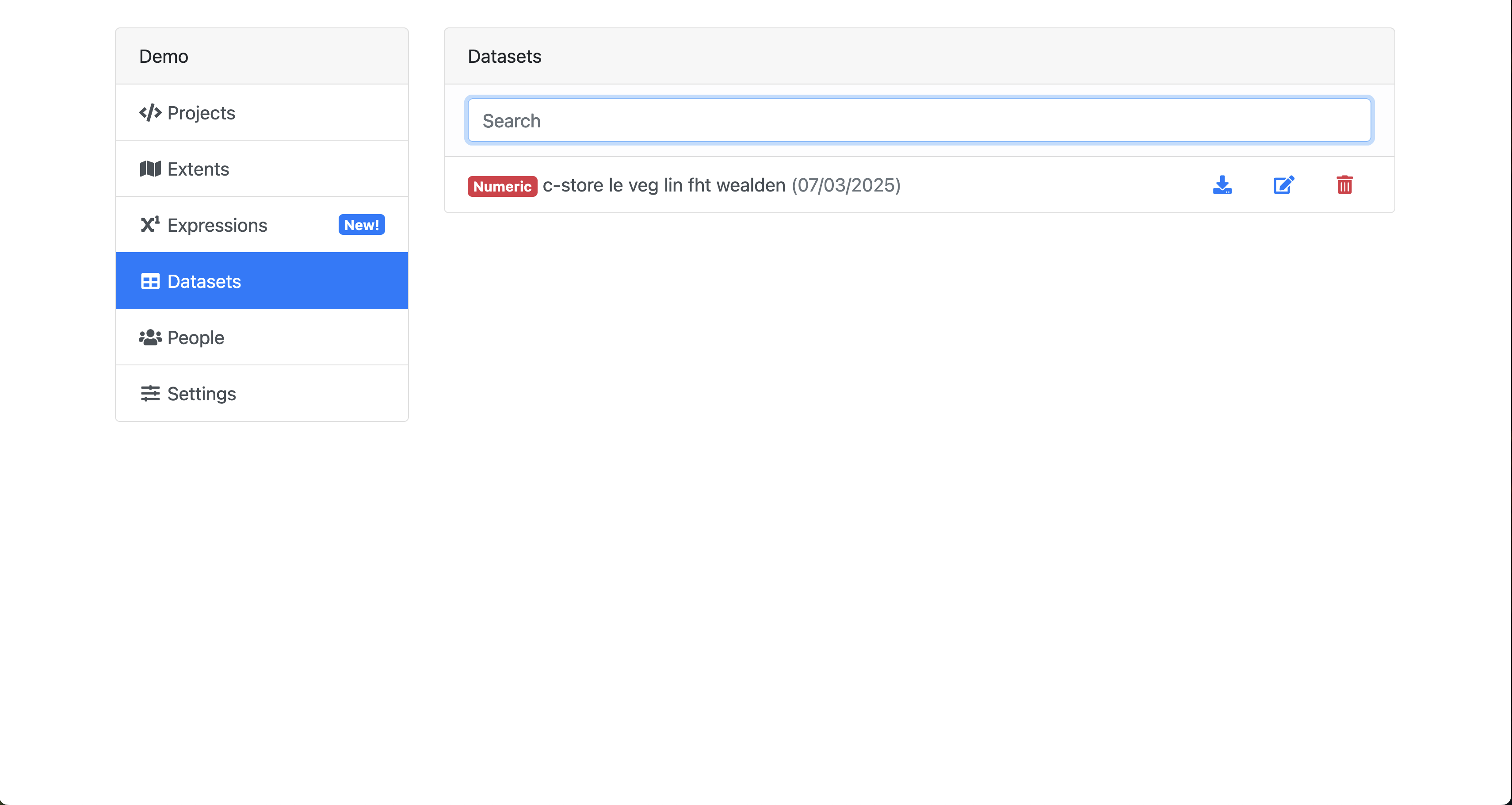
From here you can edit the name of the dataset, delete it or download it as a json file.

2.10 Using datasets in models

Next, return to the projects menu and open the “Test Project” we created at the start of this chapter and toggle Model view. Right click the model canvas and select from the “Inputs” list the component called “Load dataset.”

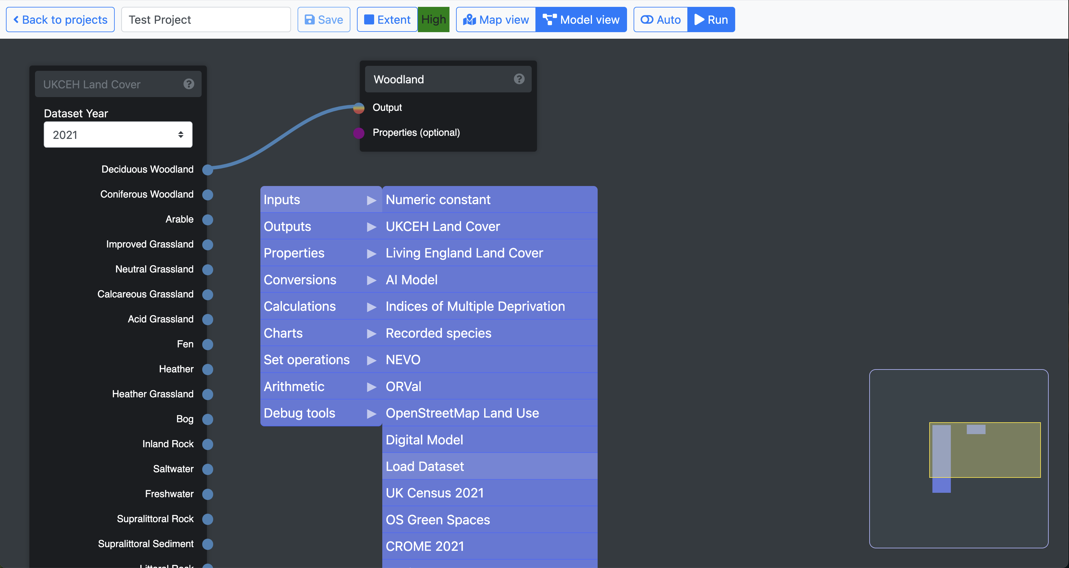
This component has one output node and a dropdown list from which to select your pre-saved dataset.

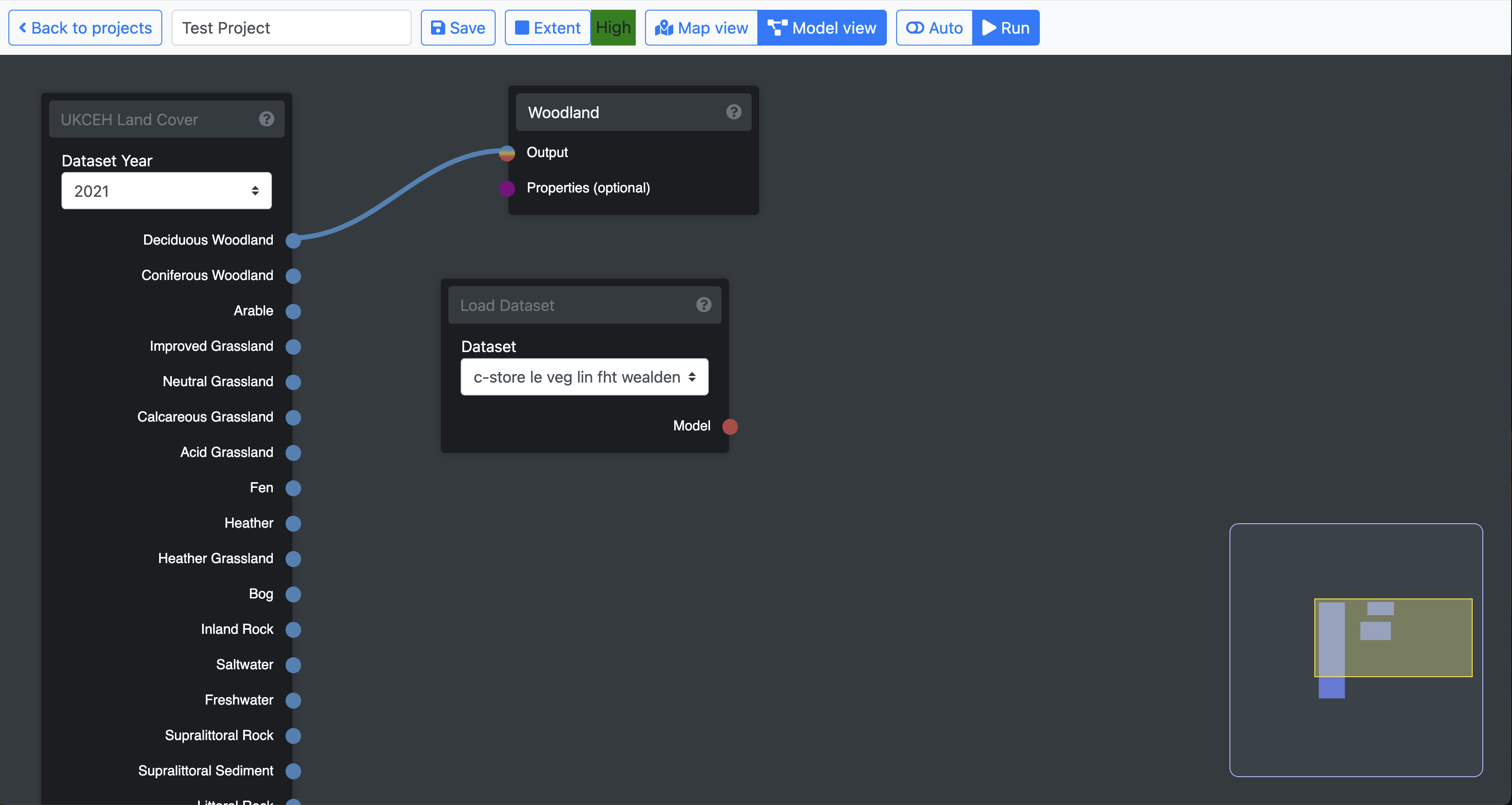
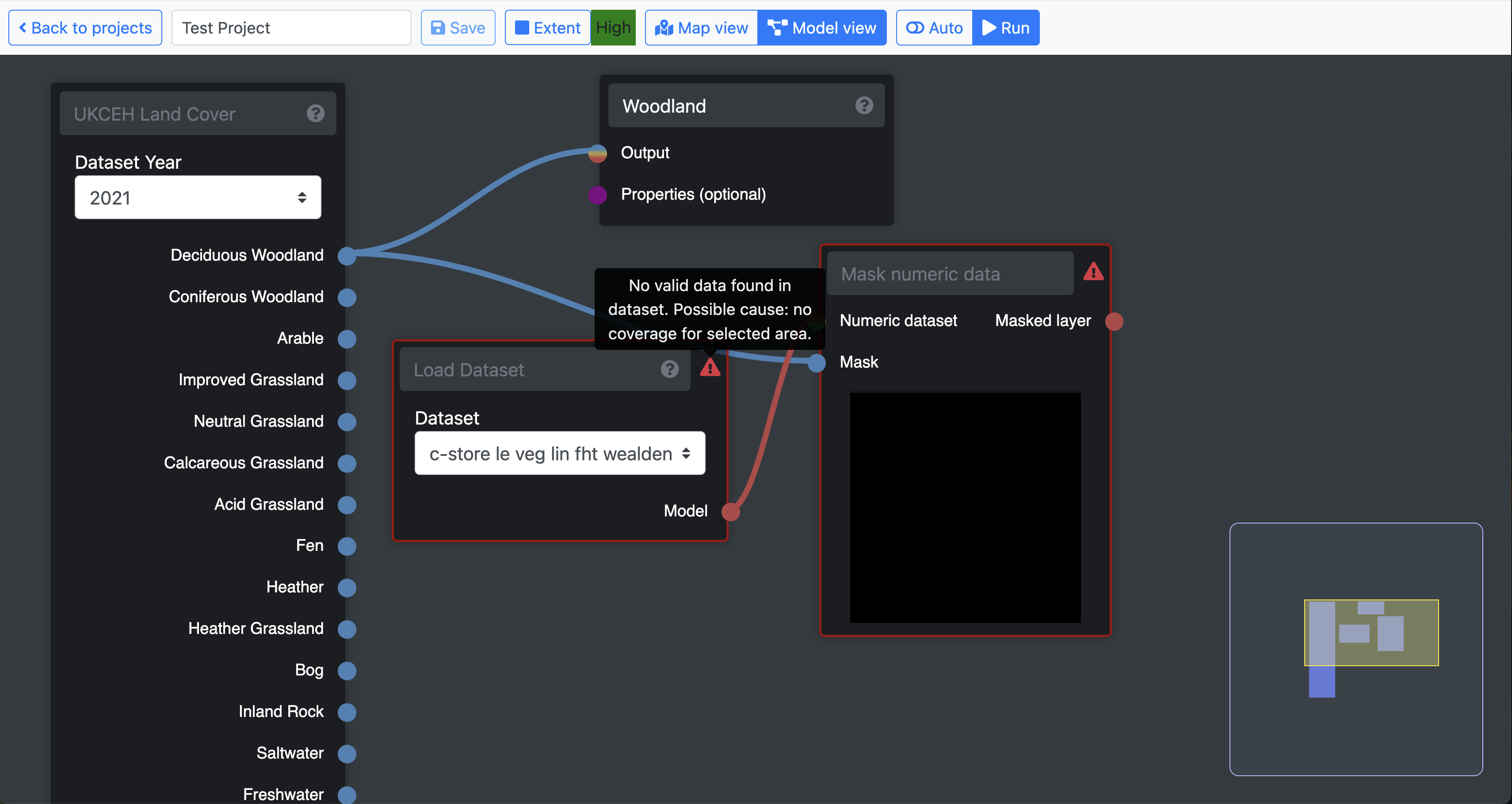
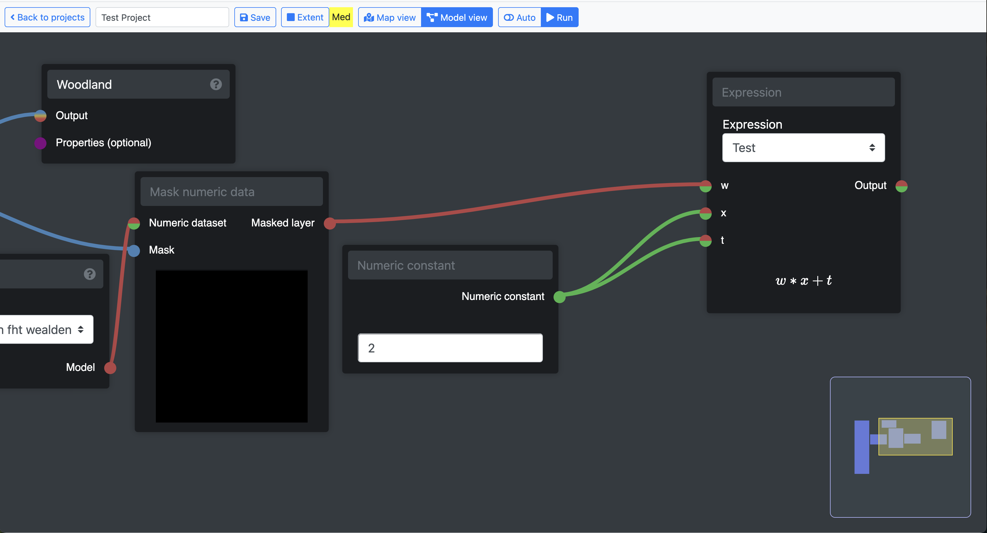
There is one very simple operation we can do first to demonstrate how to use the dataset in a model. We will use the Deciduous Woodland class from UKCEH to mask the c-store dataset thus creating a map of carbon stored in one type woodland.

First, select from the “Arithmetic” list the component called “Mask numeric data.”

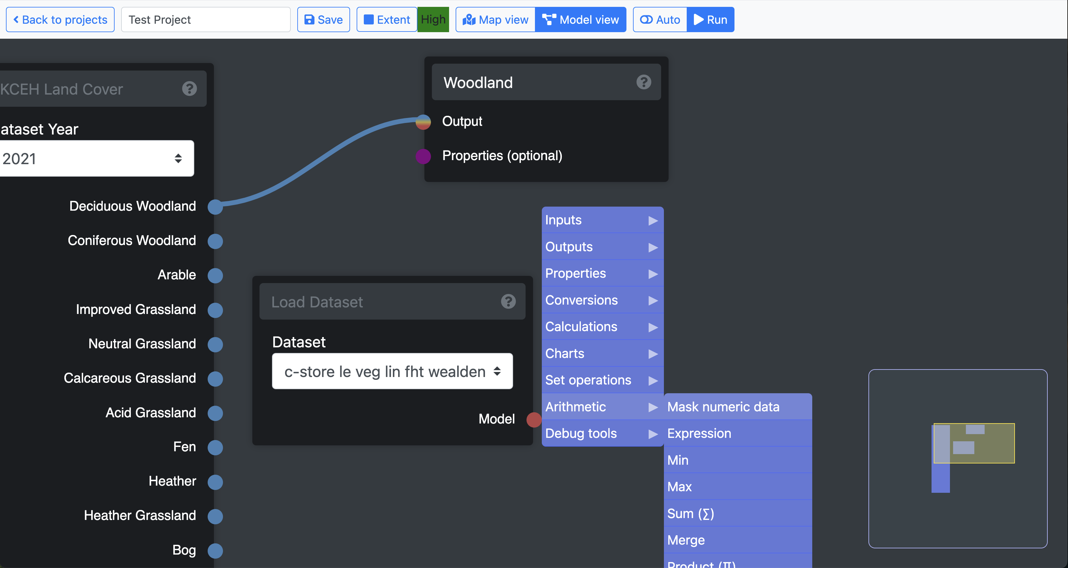
This component takes two inputs (a boolean layer to provide the mask and a numeric dataset to be masked) and provides one output (masked layer).

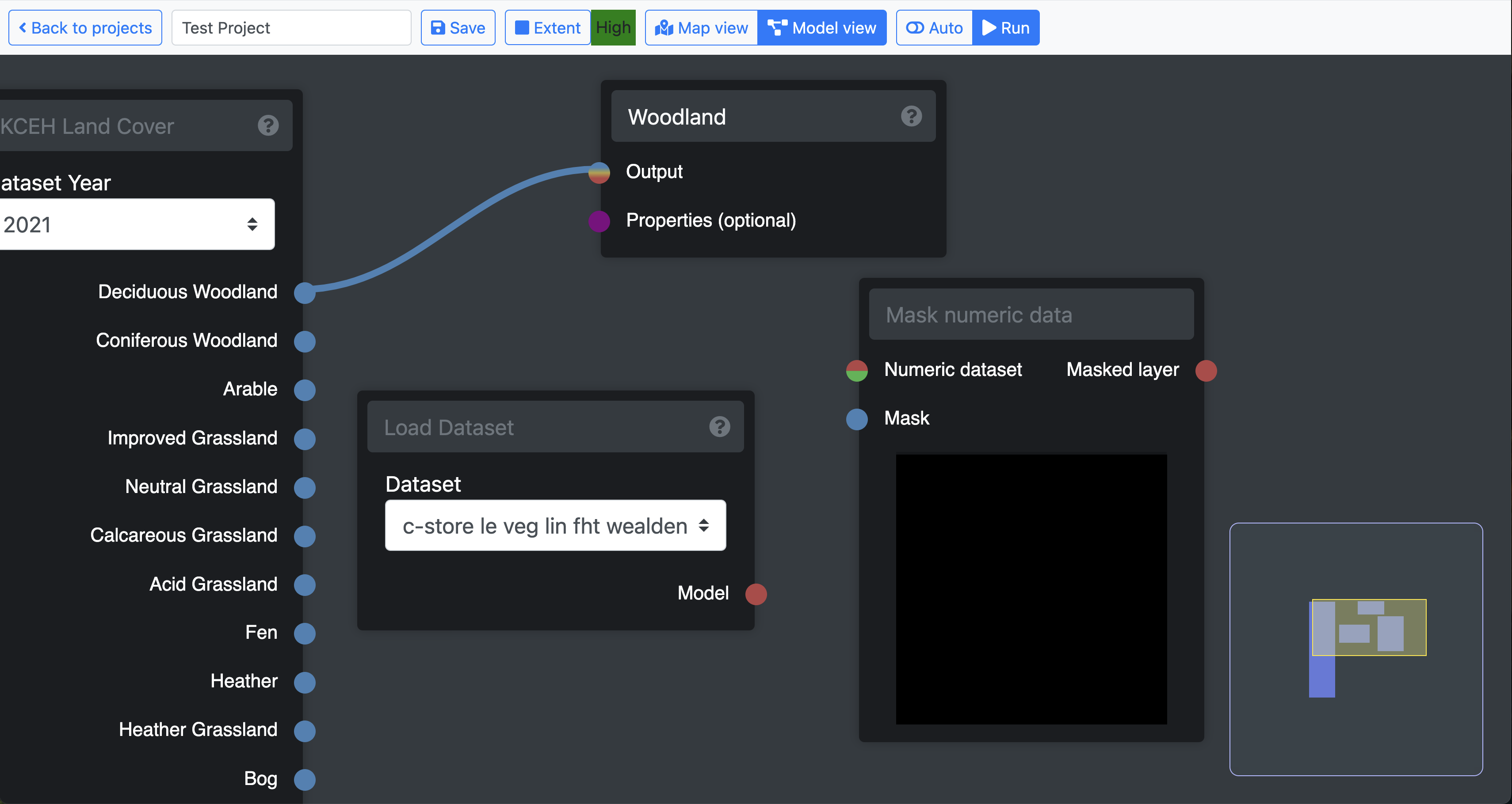
Connect the output from the loaded dataset to the red node labelled “Numeric dataset.”

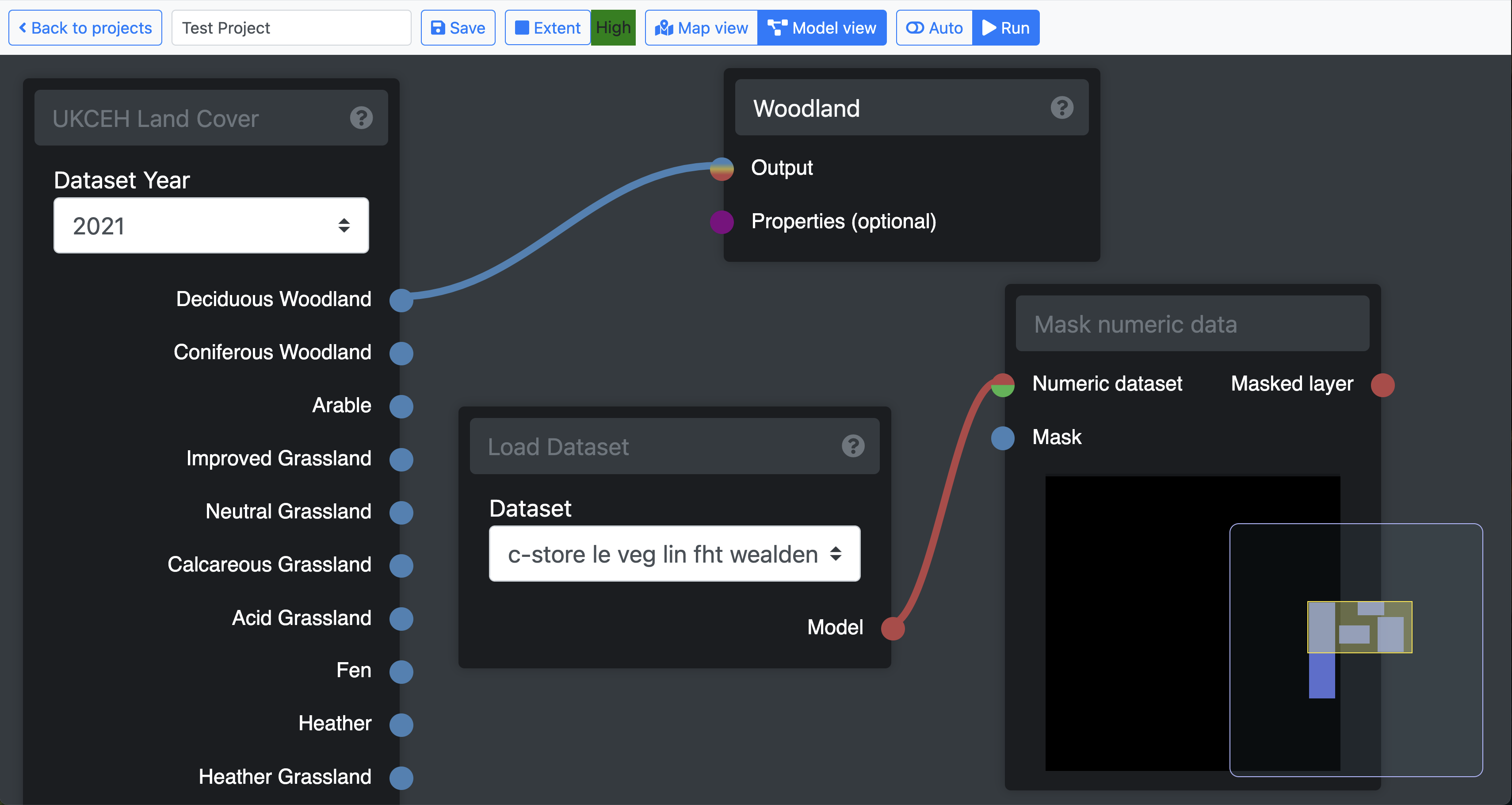
And connect the Deciduous Woodland node to the blue node labelled “Mask.”

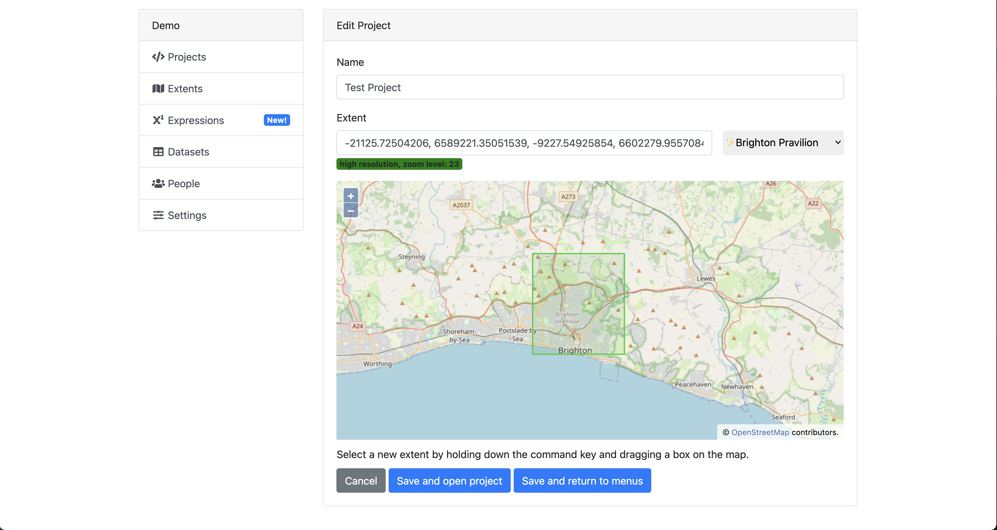
If you run the model now it will fail to execute because the dataset does not cover the same area set as the project extent. It was created for the Wealden District Council exent and this project is still set to the Brighton Pavillion extent.

Click the “Extent” button on the top menu bar and change the extent to match the loaded dataset.

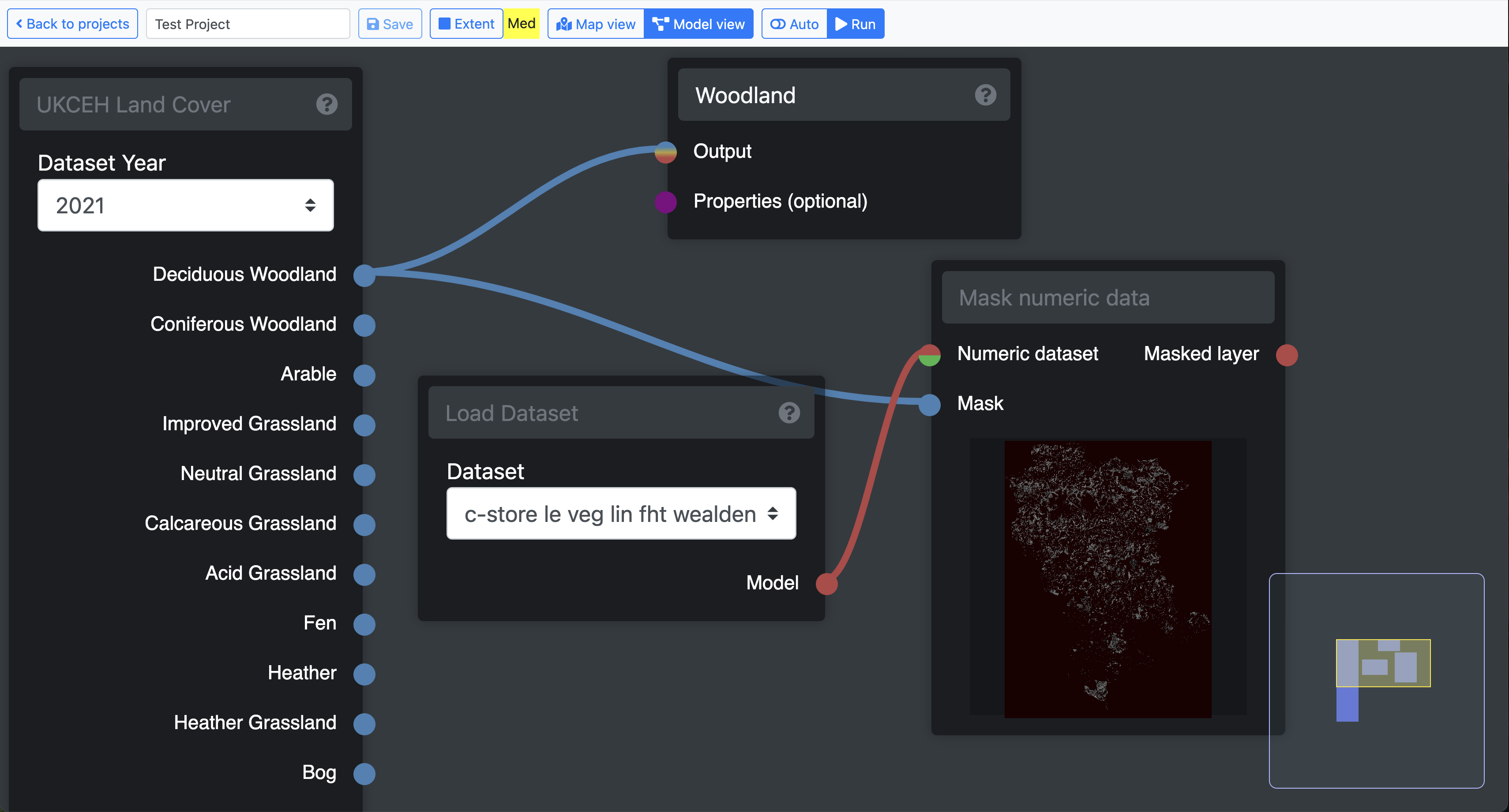
Now when you run the model it should produce a preview inside the “Mask numeric data” component so that you can verify that it is doing what you expect.

The new masked layer can be added to Map view or saved as a new dataset in the same way as described above.

2.11 Adding datasets as map layers

Alternatively, datasets can also be added directly in Map view as new map layers. Your saved datasets are displayed under the dropdown list labelled with your team name. In this case “Demo.”

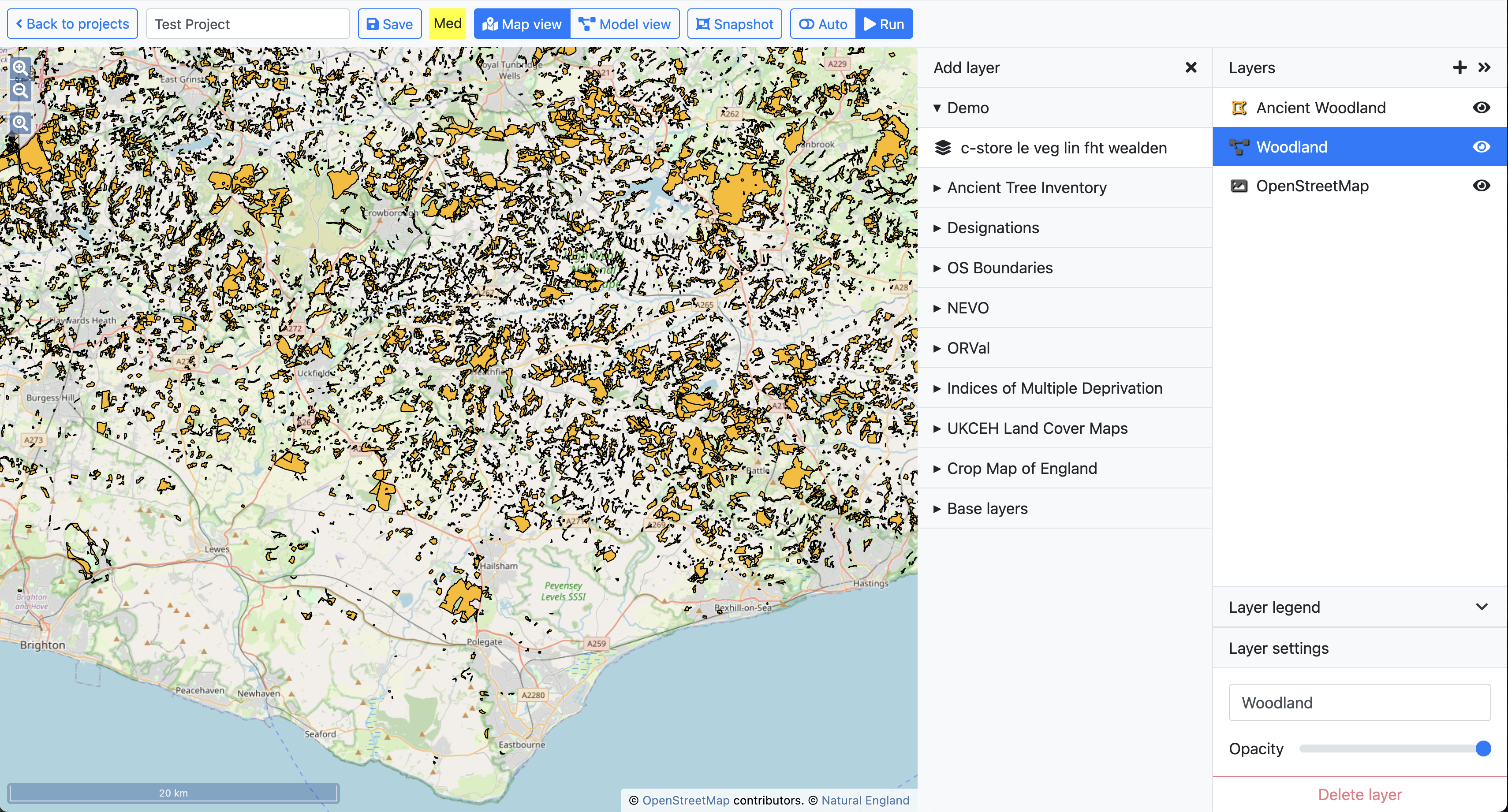
As soon as you select the dataset it will be added to the layer list and displayed on the map.

The fill mode of the new dataset layer can be changed in the same way as a layer added directly from Model view.

One key difference with pre-saved datasets is that they load directly when you open the project whereas layers added directly from Model view using the “Map layer” component are only visible after running the model.

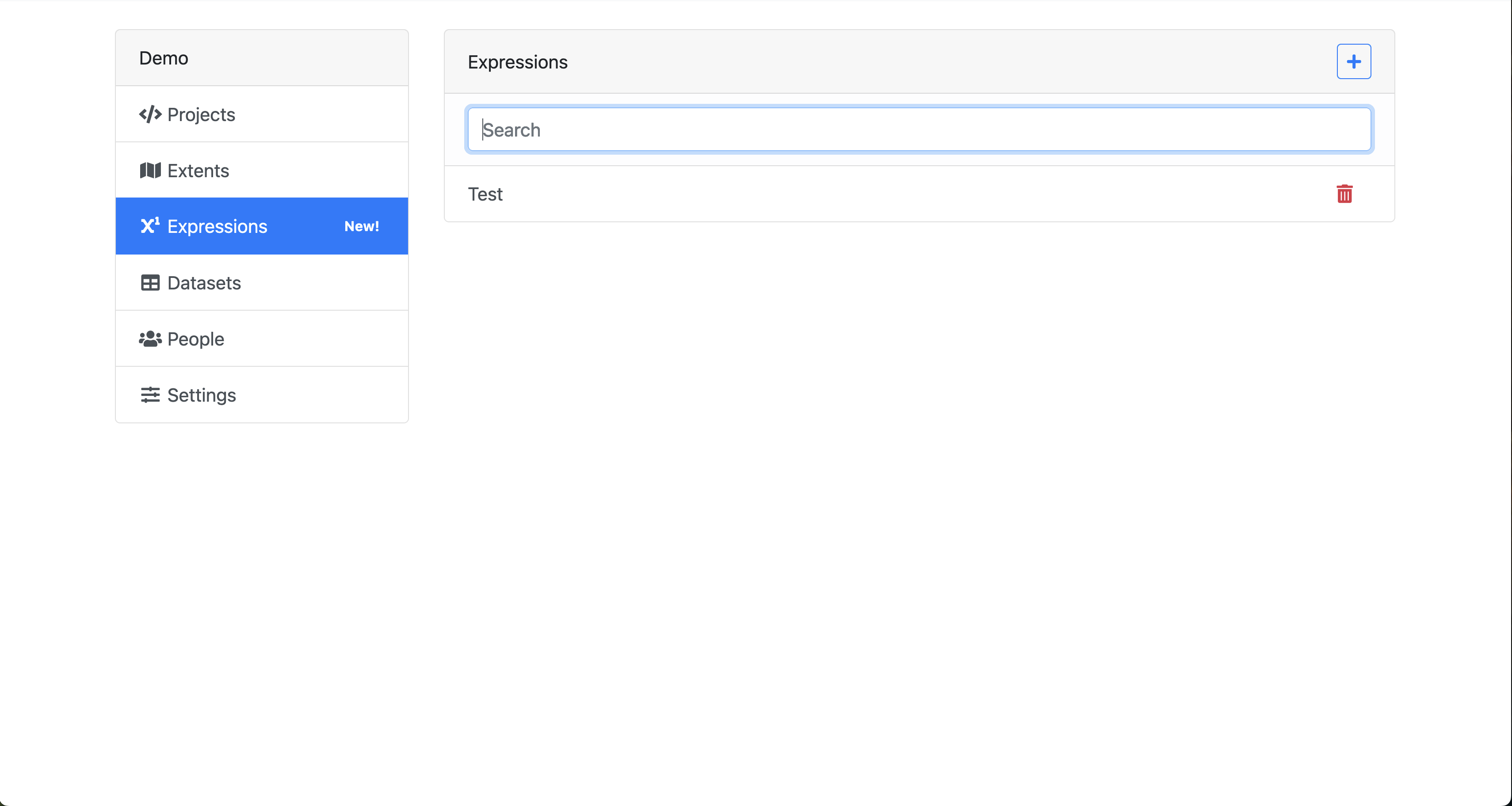
2.12 Expressions

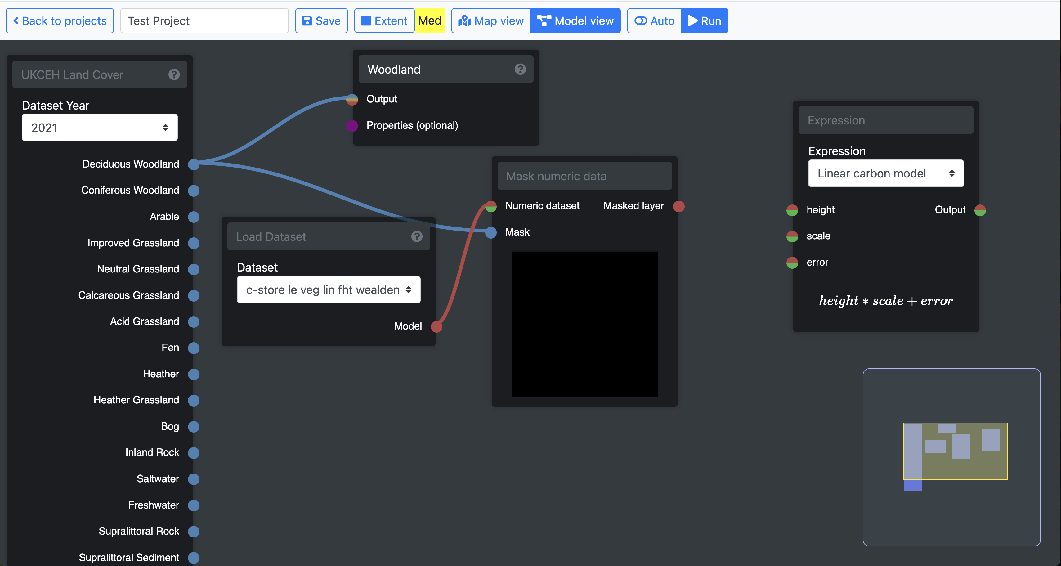
There is one more very important component that can be used in Model view and which provides a great deal of flexibility for building your models. It is the “Expression” component and you can find it in the “Arithmetic” list.

This component has a number of inputs (which are adjustable as you will soon see) and generates one output. It also has a drop down list for you to select from a choice of different expressions.

Before we use this component in the model we can create our own expression from the expression menu in project view.

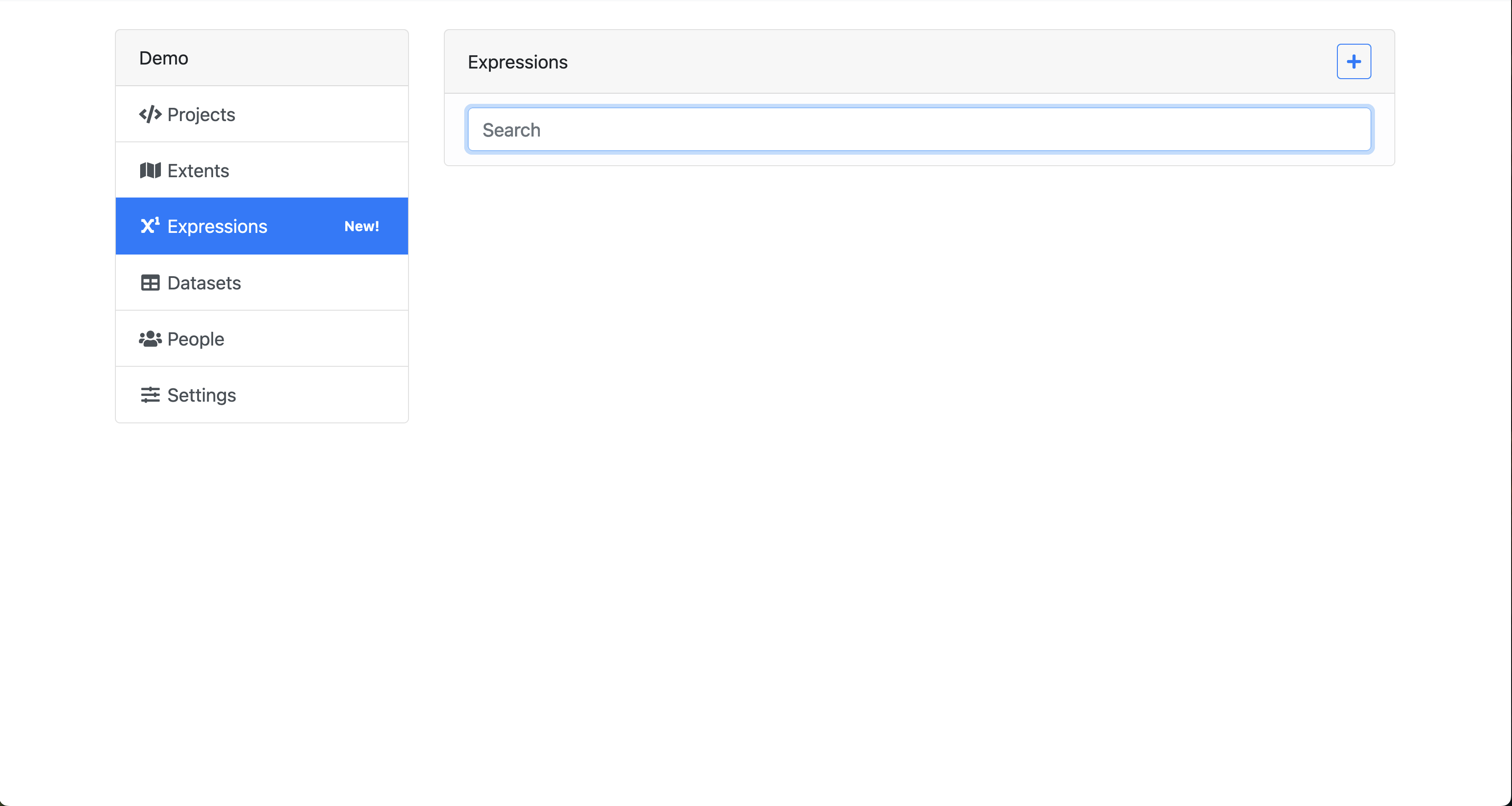
Click the blue “+” sign to create a new expression.

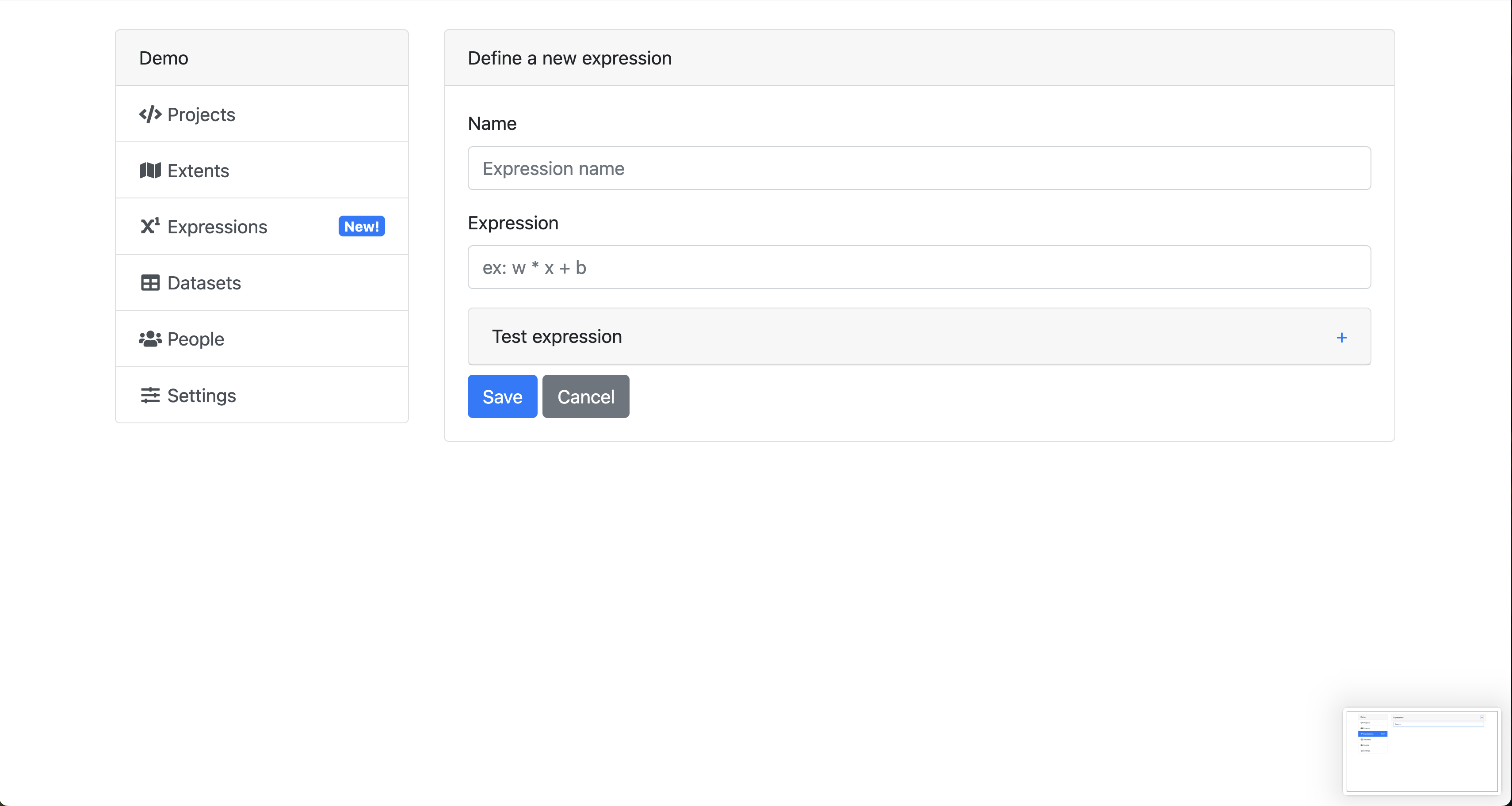
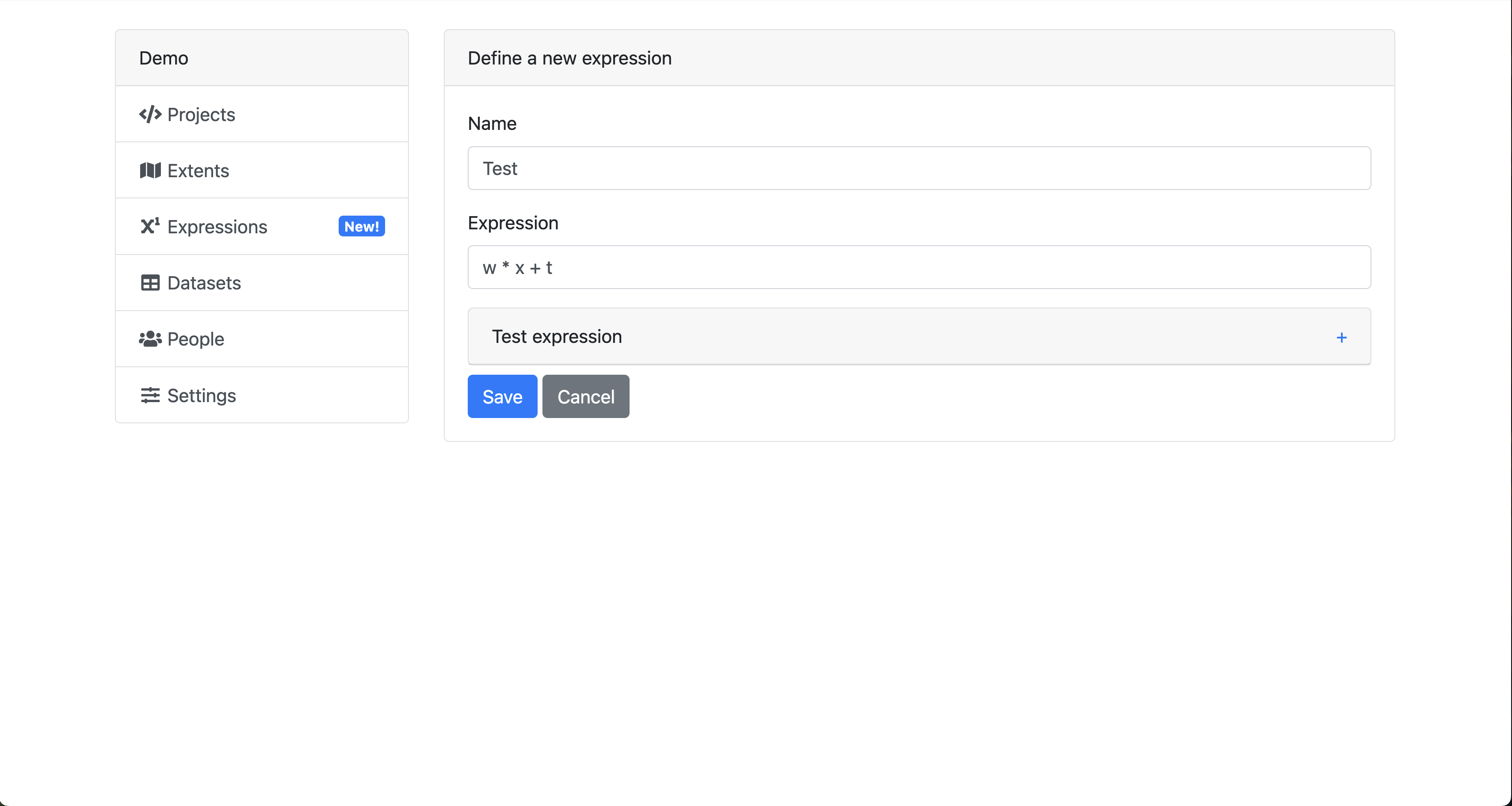
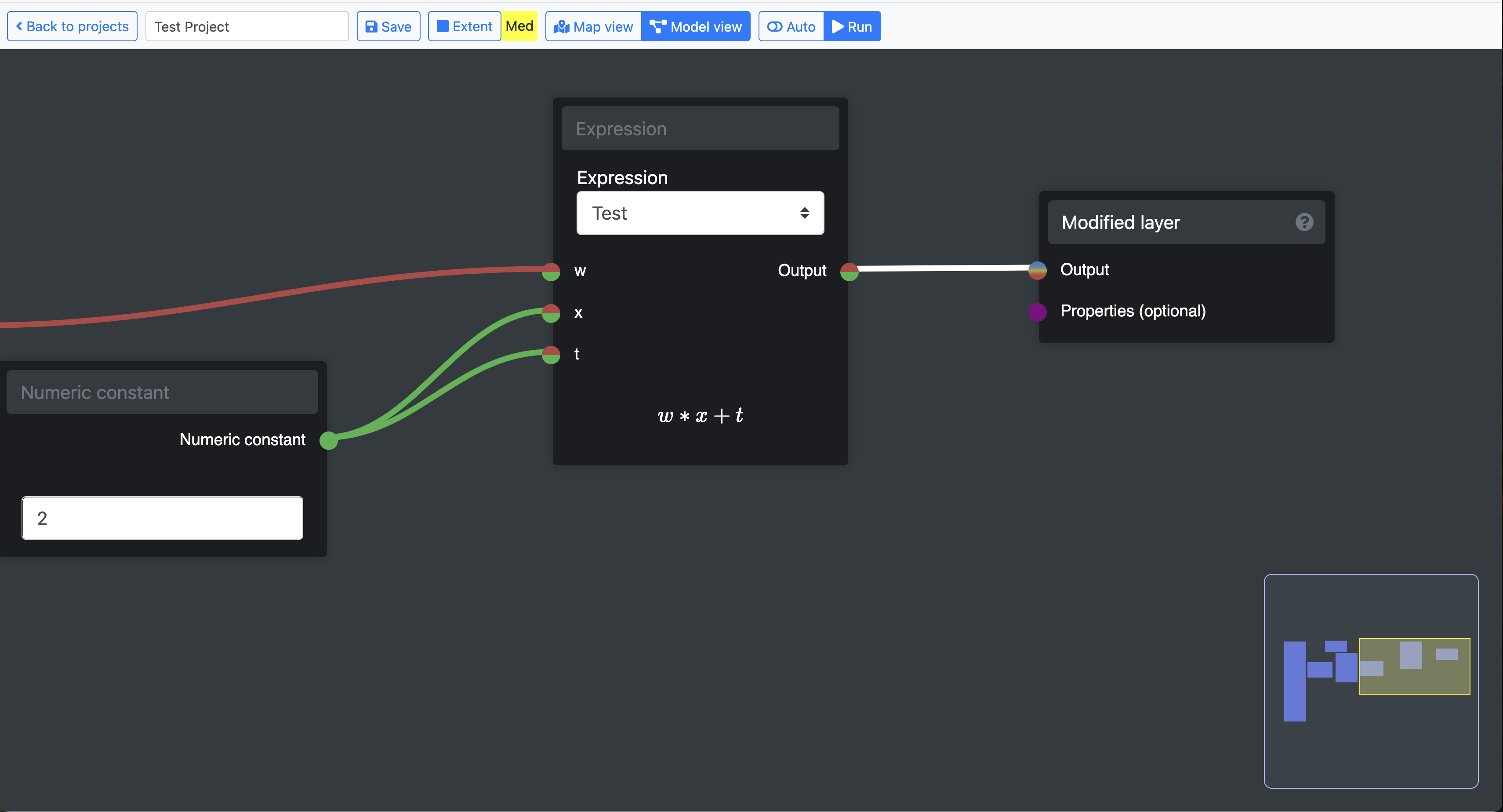
Here we can name and define our own expression. For now we can simply call it “Test” and define a simple formula “w * x + t”. This will create an expression component with three inputs corresponding to the text in this formula which will perform the calculation as defined for each cell in the input dataset to provide a equivalent output dataset.

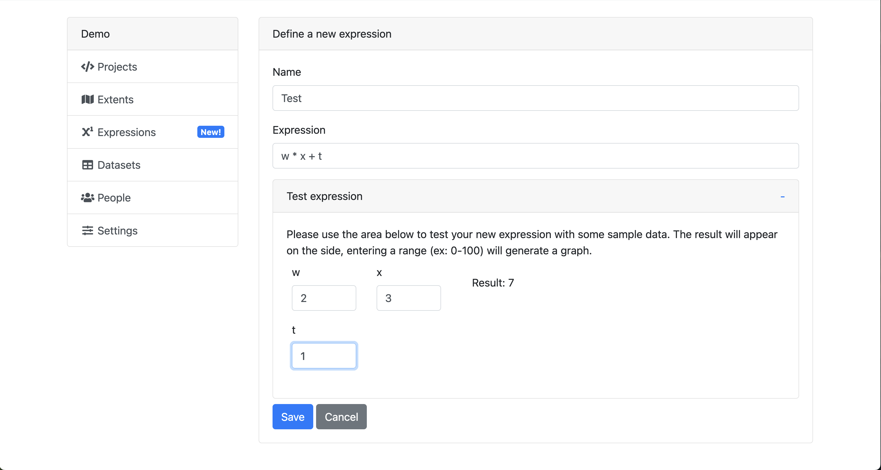
To check that the expression is doing what we expect we can click the “Test expression” button and enter some numbers to view the result.

Save the expression and you should now see it listed in the Expressions menu.

Return to the project and toggle Model view. You should now see the new expression that we just created in the drop down list of the Expression component.

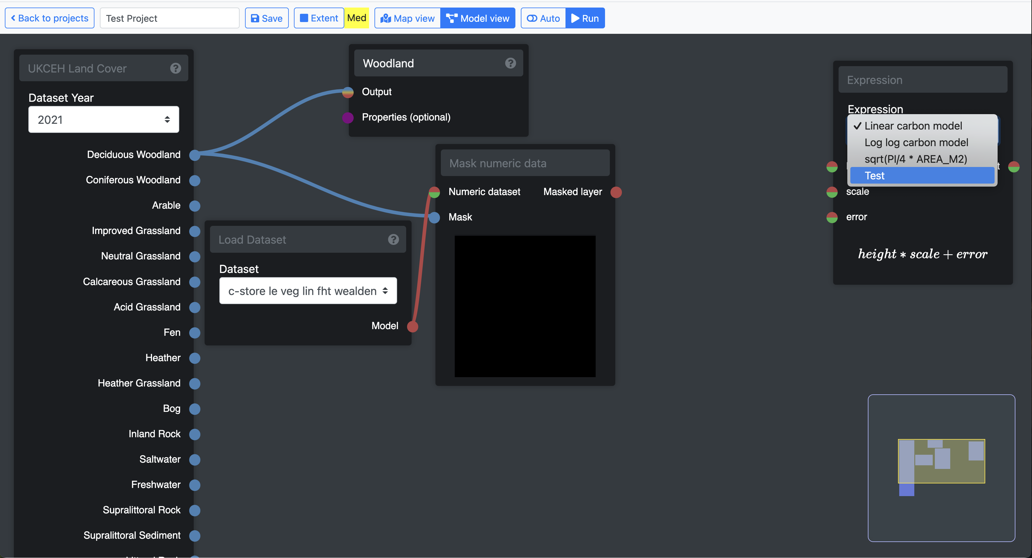
When you select the “Test” expression, the component box will change to create the correct input nodes and display the formula to show you the calculation it will perform.

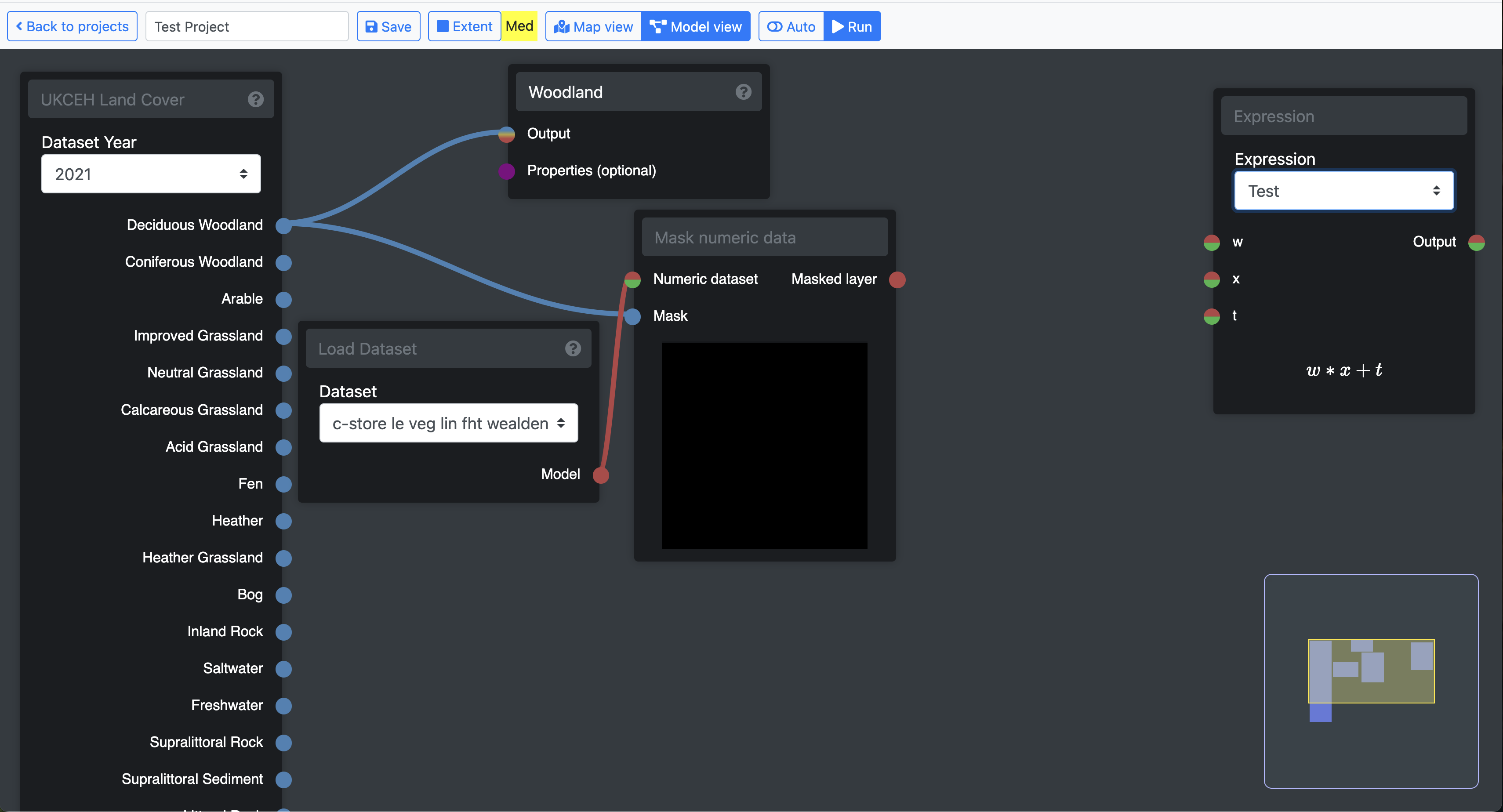
Connect the red “Masked layer” node to the expression’s input node labelled “w”.

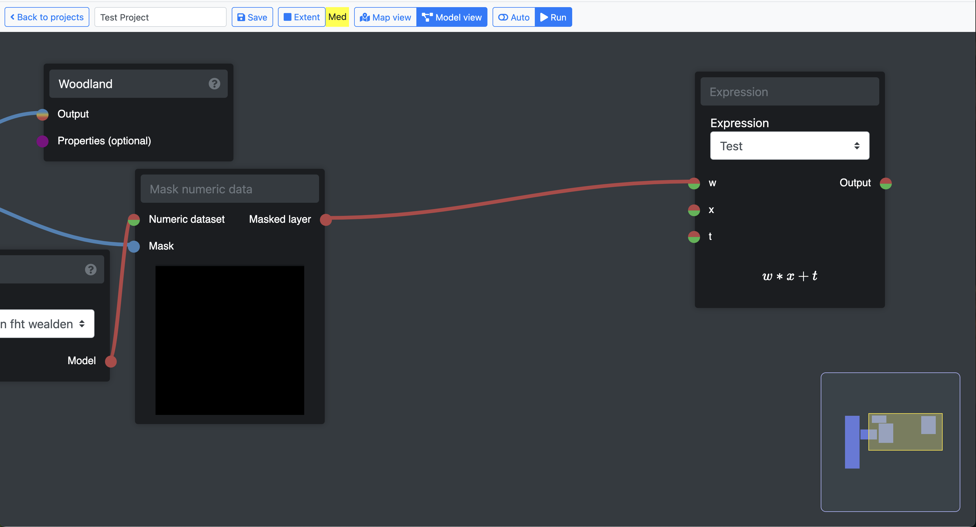
Next we can use a numeric constant to provide inputs to the other nodes “t” and “x”. You will find the “Numeric constant” component in the “Inputs” list. For simplicity’s sake let’s just connect it to both input nodes and give a value of “2”.

Finally, add a “Map layer” component to add the expression output to Map view and label it something meaningful.

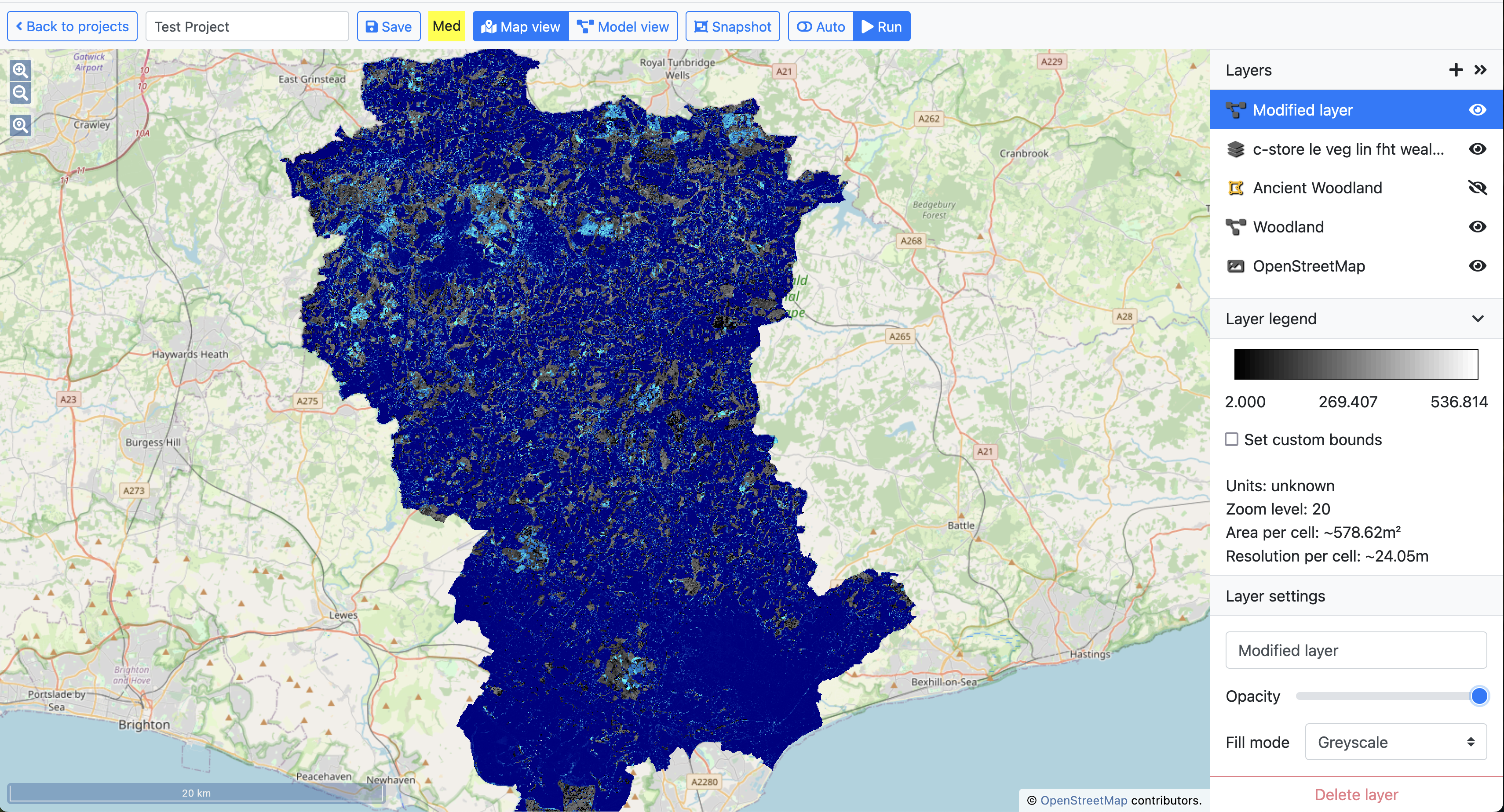
Save the project, toggle Map view and run the model to view the new map layer. You should now see it listed in the layer menu above c-store layer we added previously.

Now you are ready to play around building models and exploring your datasets alongside other map layers. For an example of use case with step by step guides to building a complete model turn to the next chapter.