1 Key Features
Our purpose in developing the LIMMMA platform is to support landscape management and planning by accelerating engagement with emerging evidence in transparent ways. The platform is designed to be flexible, accessible and extendable. Its flexibility means it can be tailored to a diversity of use cases such as mapping carbon storage and flux, biodiversity impacts, nature based solution opportunity maps, social-ecological outcomes of land-use change etc. Accessibility is vital to ensure that it is not an exclusive platform for experts but can be used by non-experts and can be used to make analysis transparent to a diversity of stakeholders. Finally, LIMMMA is designed to be readily extendable as new use cases are developed and as new features are required.
The currently live key features are as follows:
- Work with multiple datasets and map layers and add new data as required.
- Design multiple models and compare results almost instantaneously as new map layers.
- Keep modelling methods and assumptions transparent to other users and stakeholders.
- Visualise and communicate uncertainty in multiple ways.
- Run models at a variety of scales and explore the predictive limits of models at different scales.
- Extrapolate and refine models using data gathered in the field.
- Explore implications of land-use change over time and space.
- Enhance maps and models with AI and Machine Learning.
- Combine biophysical and socio-economic data outputs from multiple models into composite models for analysis of multifunctional landscapes.
This chapter illustrates each of these key features with screenshots from live projects. To view live demo projects directly on LIMMMA, you can sign up for a guest account using the following link: https://landscapes.wearepal.ai. Details of how these live demo projects were created are given in chapters 3 and 4. When you are ready to make your own projects you can simply create a new team and start building maps and models using the pre-loaded open access layers and datasets.
If you prefer a video walkthrough you can watch the video below. Otherwise, continue to the next section which provides the same content as the video in the form of text and images.
1.1 Datasets and Map Layers
The default view in a LIMMMA project is ‘Map view’ with a pre-loaded Open Street Map layer so the user can easily orientate themselves. Other map layers can be added to a project’s Map view simply by selecting from a list of available layers of different types.
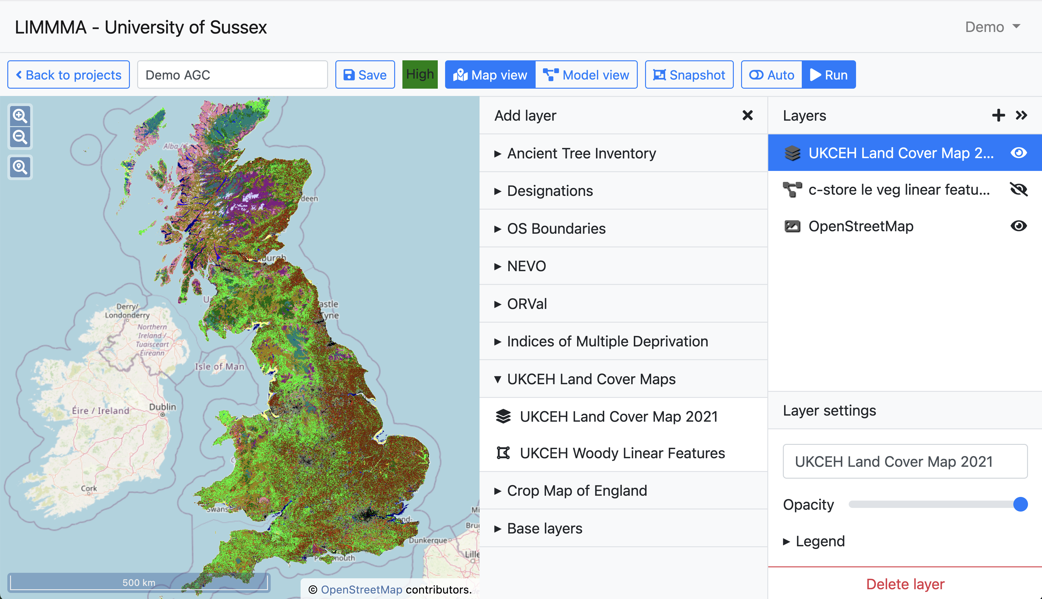
The current live version of LIMMMA includes by default the following open datasets for use by any team either in Map View or in the Model View interface:
- Ancient Tree Inventory - hyperlinked point data.
- Designations including (e.g. of ancient woodland, AONB) - vector data.
- OpenStreetMap Land Use - vector data.
- OS Boundaries (e.g. district councils, historic counties) - vector data.
- OS Green Spaces.
- NEVO model output maps - raster data.
- ORVal (e.g. paths, beaches, access points) - vector and point data.
- Indices of Multiple Deprivation - vector data.
- UKCEH Land Cover Maps for 2021, 2022 and 2023 - converted from vector to raster.
- Living England Land Cover - converted from vector to raster.
- CROME Crop Map of England 2021 - hexagonal tessellation.
- Natural Biodiversity Network Trust Atlas.
- UK Census 2021 - multidimensional vector data.
- ISRIC Soil Data.
- plus any new datasets created by members of your team for private use within your team.
However, this is not the limit of data that can be used with LIMMMA. The back end of the software allows for a technical support team to import additional datasets of almost any type for use as map layers and in the modelling function. For example, over the course of our most recent research project we have imported additional layers into our Central Sussex workspace on LIMMMA. They include the following:
- Soil samples and tree crown measurements from Kew Wakehurst - multidimensional point data with additional metadata.
- Natmap Soil Carbon datasets - multidimensional raster data.
- High resolution aerial imagery for an area of Sussex.
- Digital terrain model LIDAR Maps - hi-res raster data.
- Hedgerow maps.
1.2 Models and Outputs
These map layers and datasets can be combined in a variety of ways to create models built using LIMMMA’s integrated graphical modelling interface in ‘Model view.’
Model outputs can be added to the project’s map view as new map layers and also saved to a database within your team’s workspace for use in other projects and models.
1.3 Transparent Assumptions and Methods
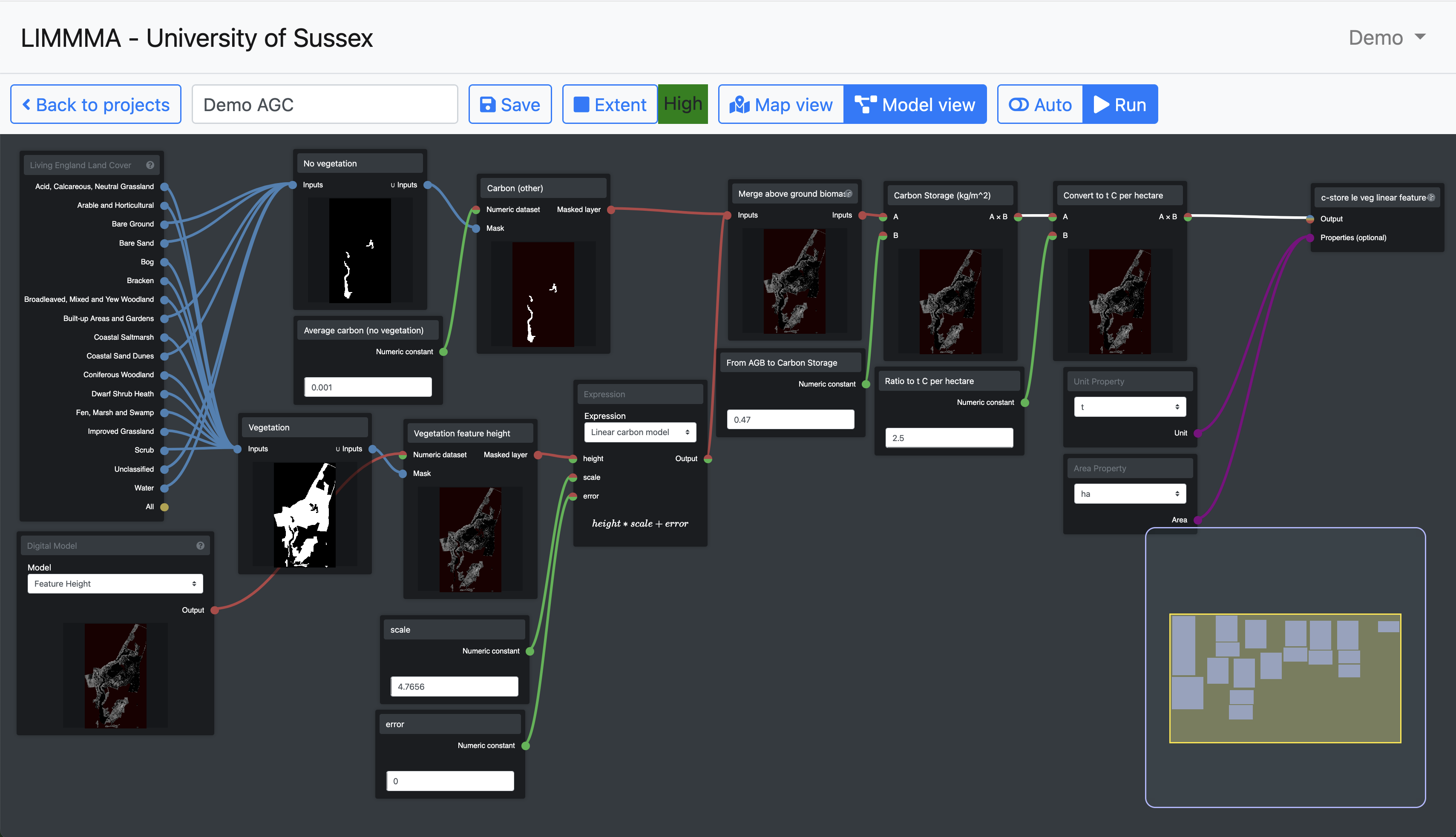
The model view interface is designed to enable users to create models that are relatively transparent, easily reproducible and make the modelling assumptions as obvious as possible to other users. This is achieved by using pre-configured graphical components which each display previews of the operation they perform. The user selects components from a list of different types and links them together to build more complex operations. The preview feature provides the additional advantage of making errors in method and data easier to detect and pinpoint throughout the model building process.
1.4 Visualising Uncertainty, Opportunities and Risk
In addition to loading datasets and generating map outputs, LIMMMA’s modelling interface also provides components which enable the user transform different types of data in various ways. Using these components in combination, a user can create new kinds of maps to, for example, visualise uncertainty in various ways or to create opportunity and risk maps to support landscape management and planning.
Identifying and estimating uncertainty
The LIMMMA team is developing ways in which users can visualise and understand the location and impact of uncertainty in models, illustrating how that uncertainty is propagated through the landscape modelling process. The intention is that uncertainties are propagated appropriately through a model and are traceable back to their original source, where possible.
See Section 3.4 in chapter 3 or download the full report for a detailed explanation of our method for calculating combined estimates of uncertainty and confidence-levels along with a walkthrough of how to implement this method in LIMMMA as an integrated part of the carbon estimation model. Below we summarise the basic components used in this method and illustrate their use with simple operations.
Set operations
The group of model components called “Set operations” enable the user to manipulate the LULC (land-use land-cover) datasets to generate new derivative or composite LULC classes. The LULC datasets are in the form of boolean grids - a georeferenced matrix of cells, each with a value of either TRUE or FALSE indicating spatially where one specific type of land use or land cover is or is not present. The set operations take these LULC grids as inputs and create a new LULC grid as their output, having performed one of the following set operations:
- Union joins two LULC classes (A and B) into a new LULC class in which the value TRUE now represents the entire area covered by both inputs (i.e. if a cell is TRUE in A or B or in both it will be TRUE in the output).
For example, you could use Union to combine two or more types of vegetation classes (forest, grass, arable etc.) into a new LULC set representing all vegetation in the landscape as a single class.
- Intersection creates a new LULC class corresponding to the overlap between the two inputs and returning FALSE for every cell in which the two inputs do not overlap (i.e. if a cell is TRUE in A and B it will be TRUE in the output while all other cells will be FALSE).
You might use Intersection to create a new sub-class of Coniferous Woodland which coincides with the areas covered by AONB or National Parks.
- Set difference creates a new LULC class corresponding to the area that is unique to the specified input (i.e. a cell will only be TRUE in the output if it is TRUE in input A and FALSE in input B).
This operation is useful for identifying locations where two different land cover classification maps disagree or for revealing the changes in land use or land cover between two points in time.
Symmetric difference creates a new LULC class corresponding to the area covered by two input classes with the exception of where they overlap (i.e. a cell will only by TRUE in the output if it is TRUE in either input A or input B but no TRUE in both).
Complement creates a new LULC class corresponding to the area NOT covered by the input class (i.e. if a cell is TRUE in the input set it will be FALSE in the output and vice versa).
For example, you might want to exclude all grassland cover in conservation areas from your opportunity map for projects to create new woodland.
Arithmetic components
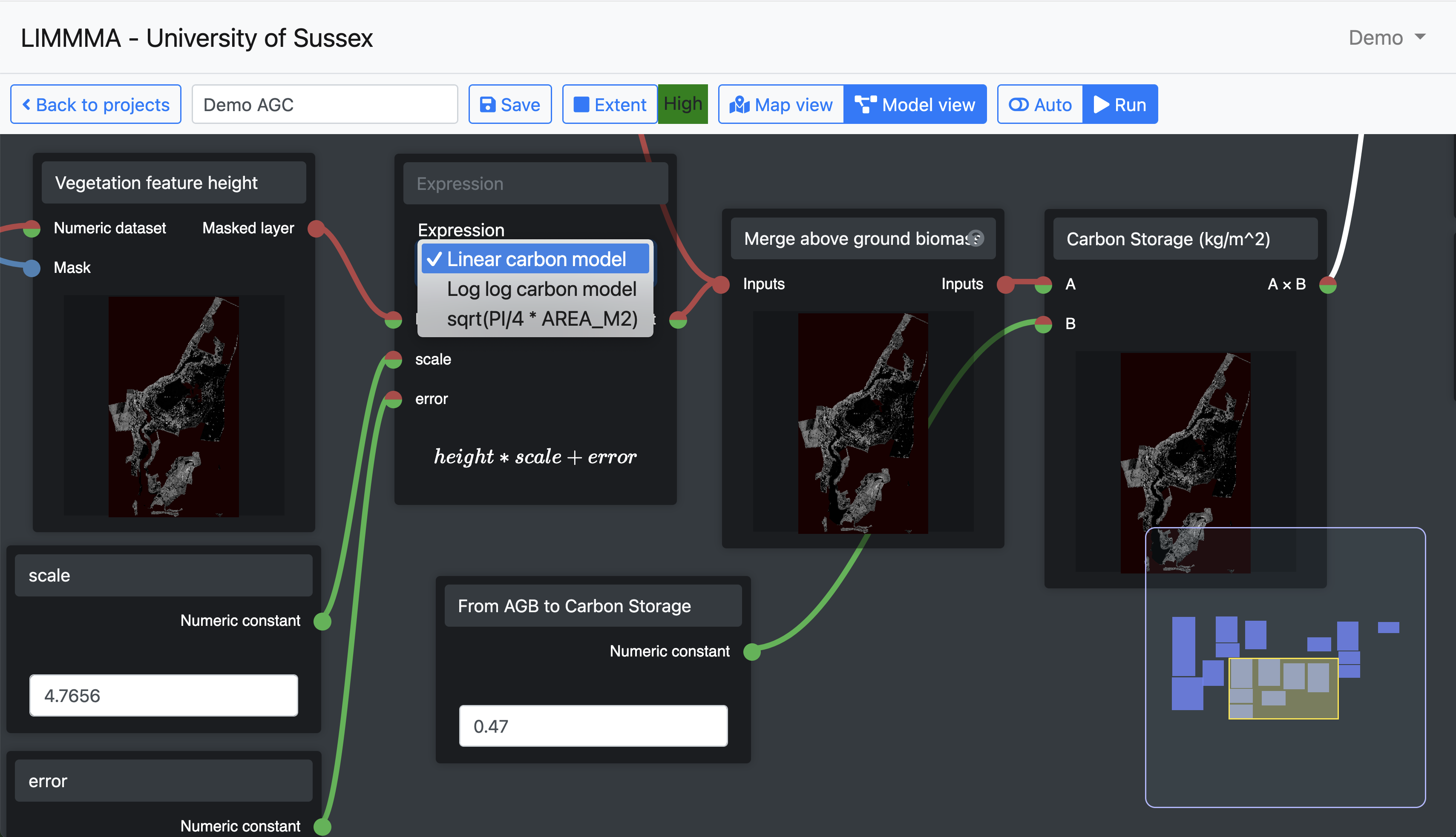
“Arithmetic” components are used to perform calculations on numeric grid data - a georeferenced matrix of cells, each with a number value instead of a boolean value. These include a range of simple operations such as add, subtract, and divide, a merge operation and a bespoke expression component which allows the user to select from a list of pre-built equations to allow for more complex calculations. These type of components are key to building models which estimate carbon storage, for example, but are also useful for quantifying the discrepancies between outputs from different models.
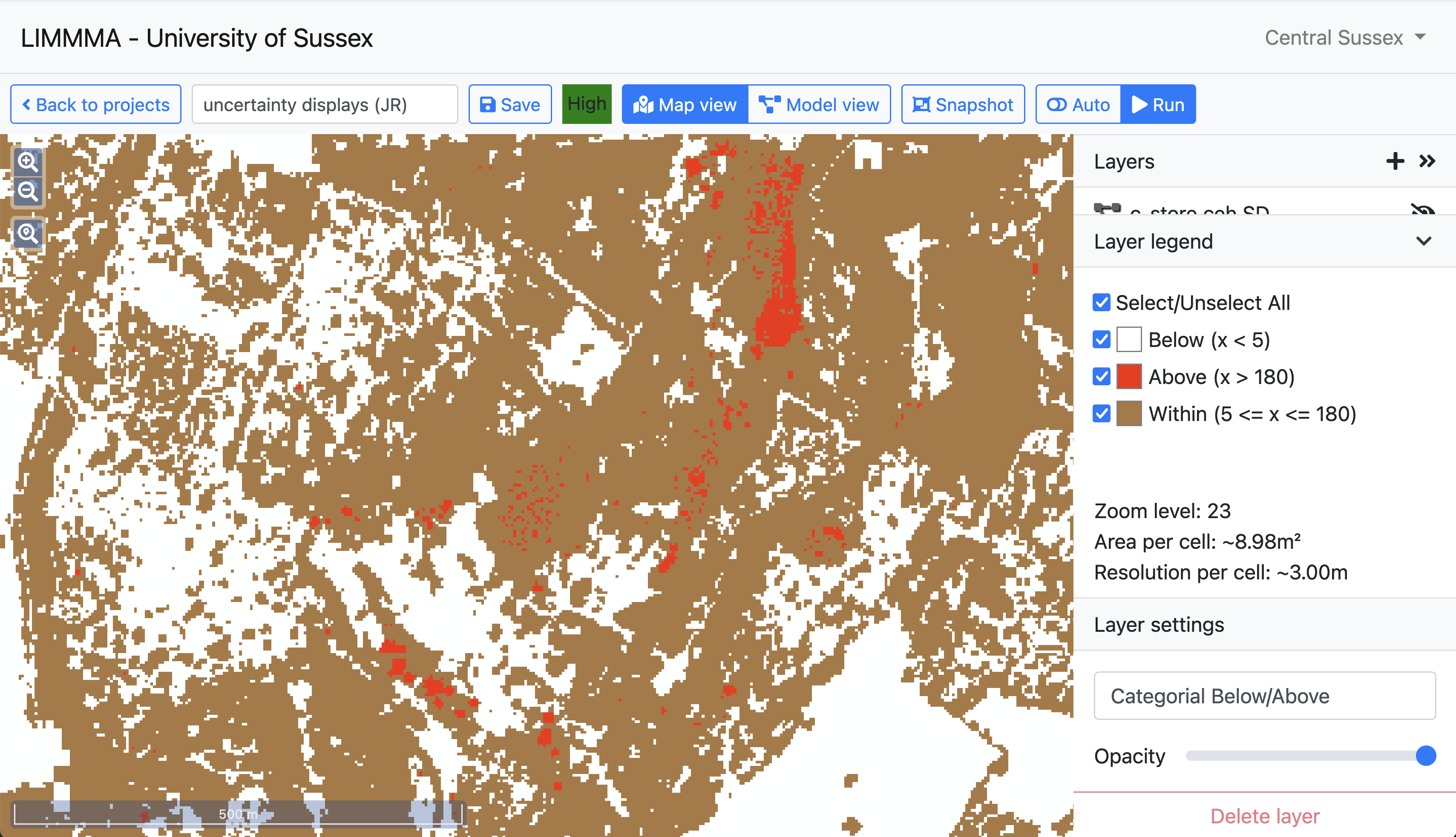
Revealing locations of uncertainty
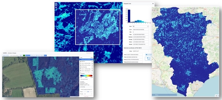
Here is an example of using the Union and Set difference components to create a map showing the disagreement between the UKCEH and the Living England Land Cover maps over classifying vegetation and non-vegetation land cover classes.
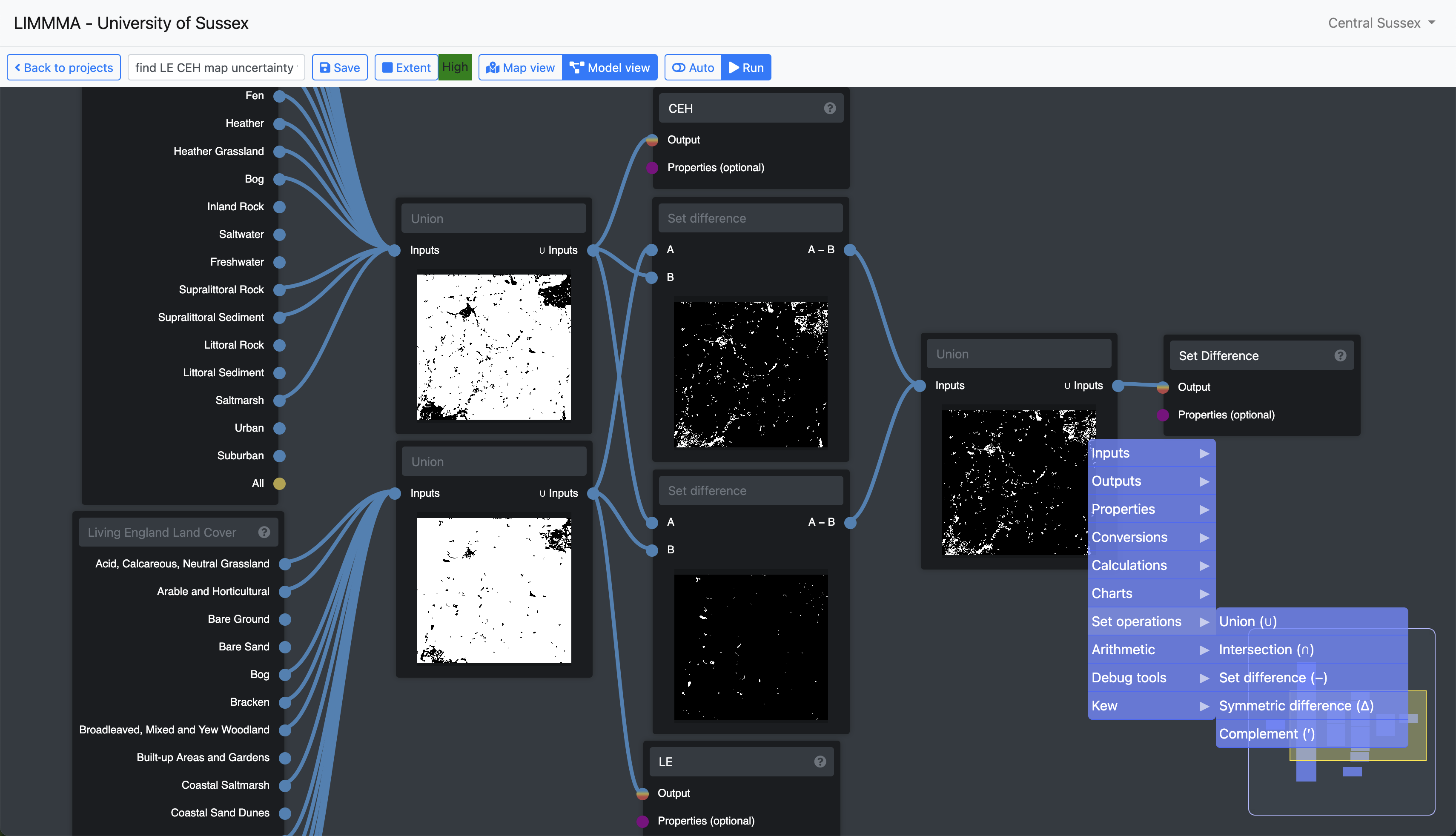
In Map View the final output of these set operations can be viewed as a new layer which reveals the potential sources of error derived from the different habitat mapping methods used to create the UK Centre for Ecology and Hydrology (UKCEH) and the Living England (LE datasets. This type of uncertainty map allows the user to pinpoint those locations where carbon estimates are subject to a higher degree of uncertainty.
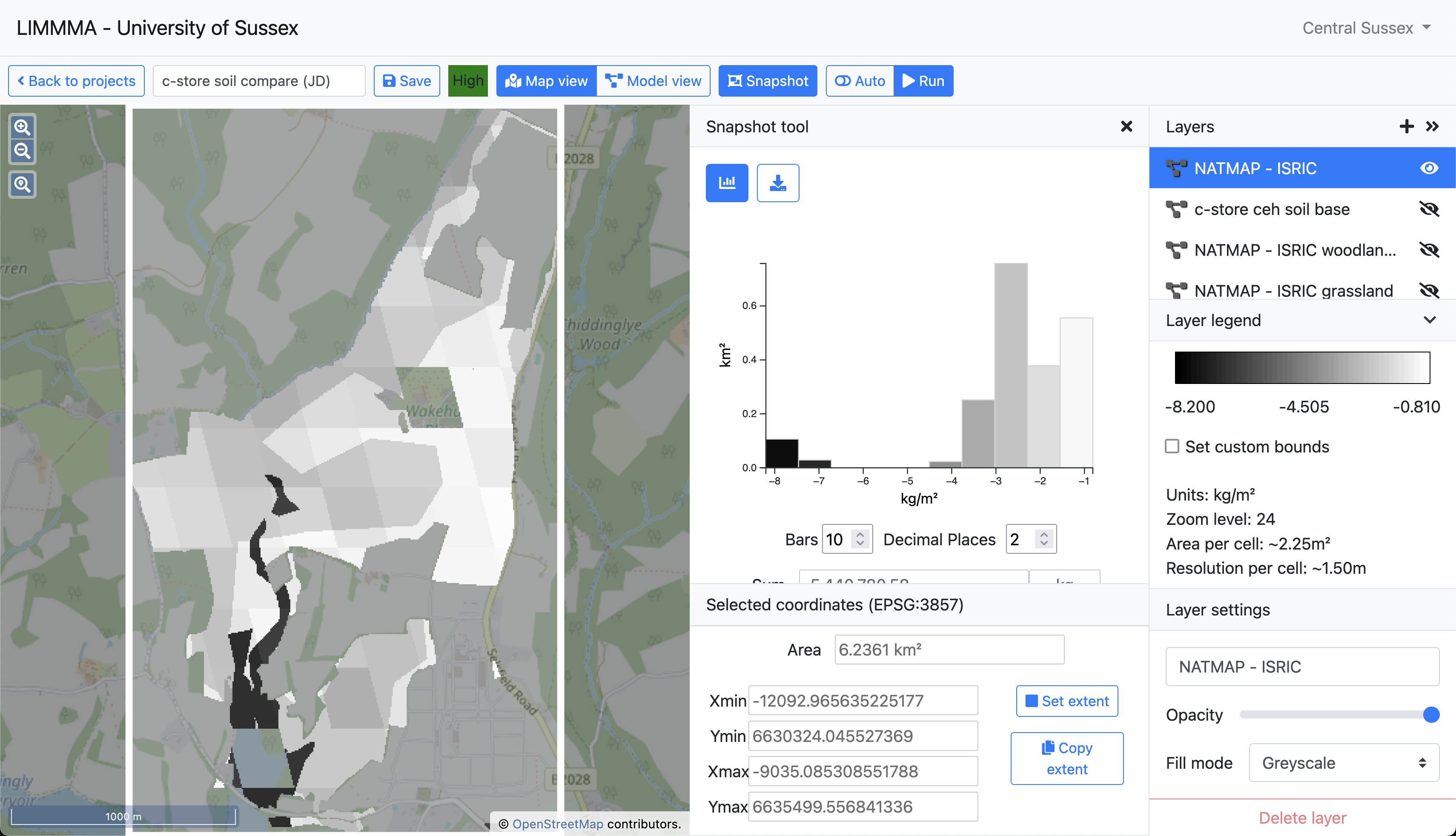
Quantifying discrepancies between models
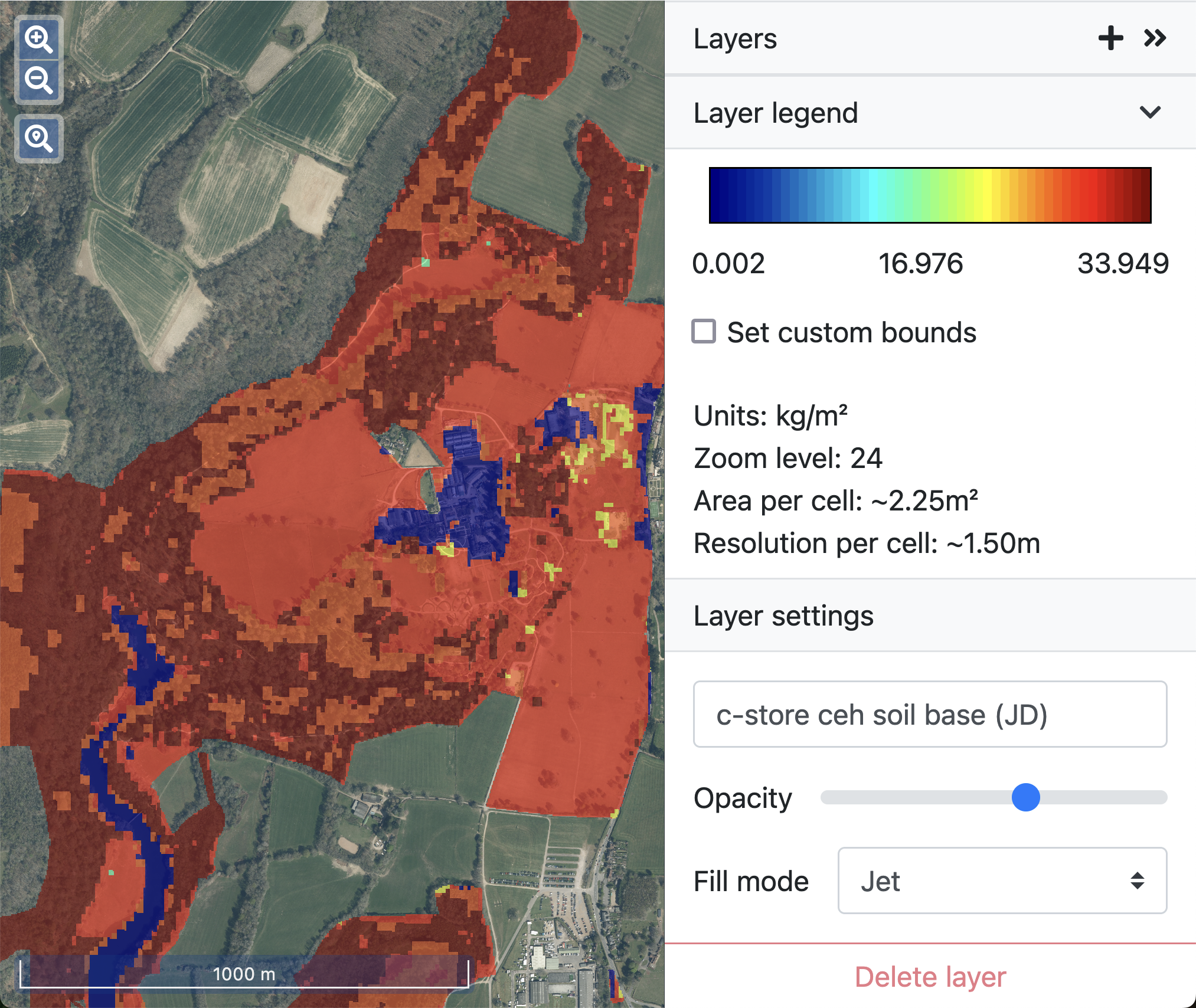
Now consider a situation in which you want to quantify and visualise the discrepancies between competing approaches to modelling a particular environmental variable such as carbon storage or indicators of soil health or biodiversity. Using the subtract component the user can map the differences in value estimates generated by two separate models for each cell in a numerical grid. Below is fragment from one such model which calculates the difference between the NATMAP and ISRIC estimates of soil organic carbon in the landscape.
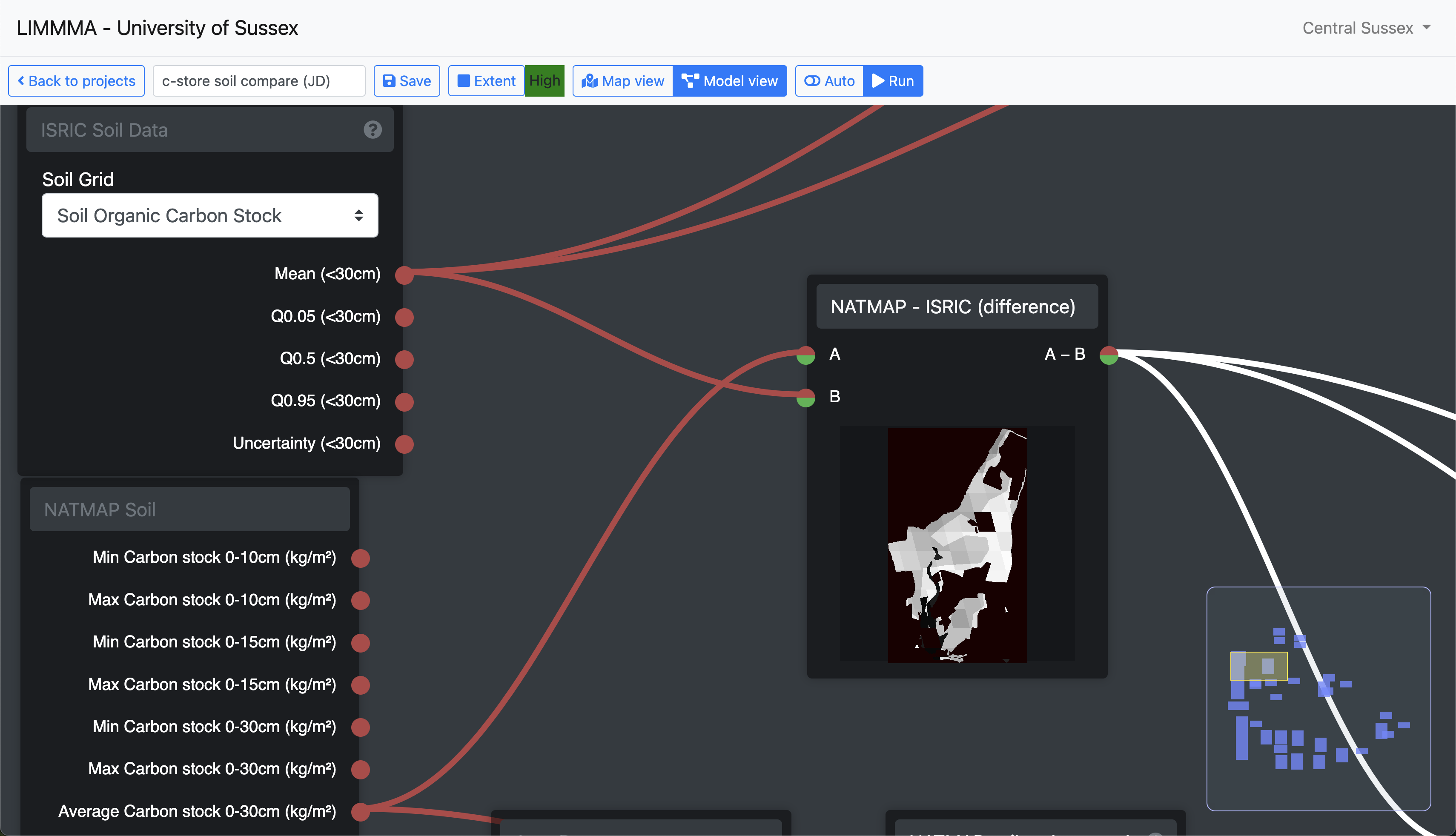
When the output is added to Map View it provides a clear picture of where the two soil maps disagree about the amount of soil organic carbon and by how much.
Opportunity Maps
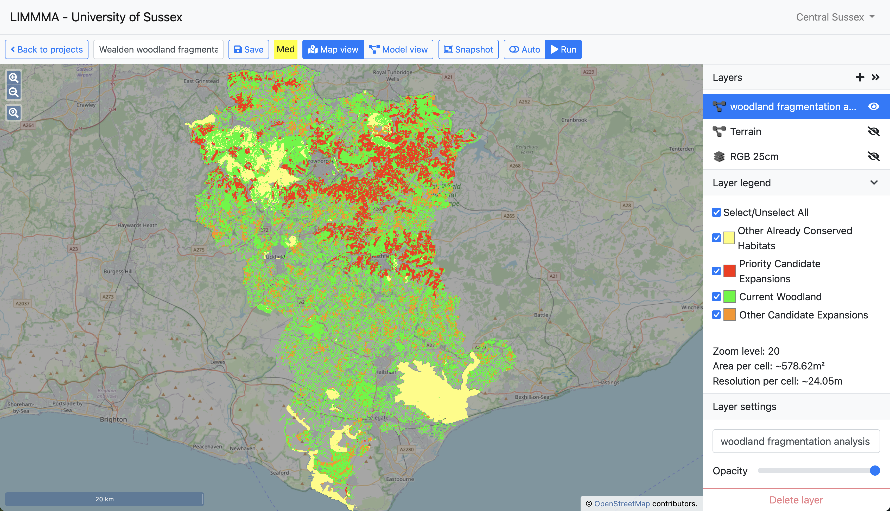
Creating opportunity maps and risk maps which display specific locations that match certain conditions can also be done using a combination of set operations and other model components. Here is a rather complex model that identifies candidate sites for woodland expansion projects.
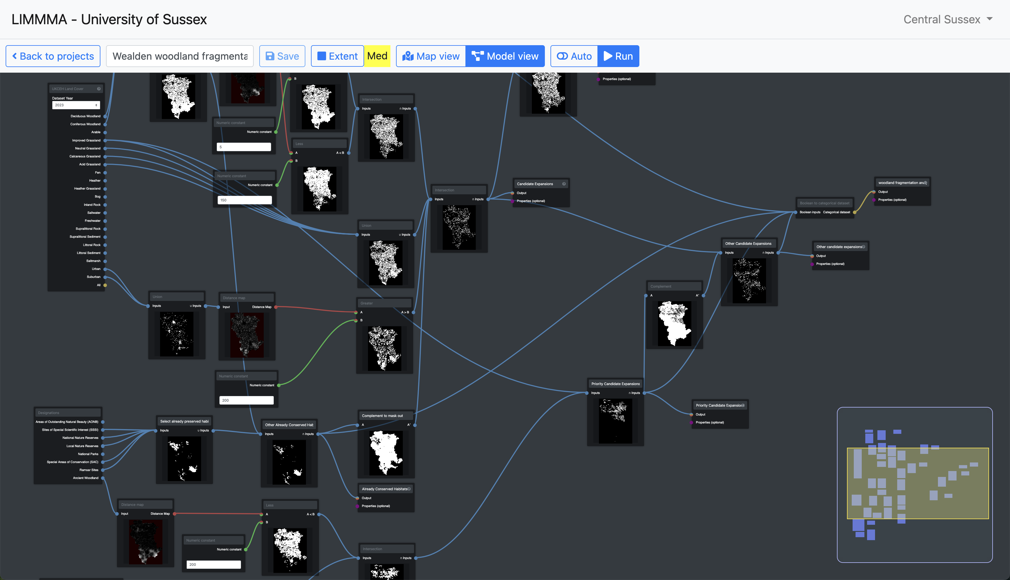
In Map View you can see how the model is designed to highlight areas with higher or lower priority for woodland expansion (in this case based on several parameters including proximity to existing ancient woodlands and location in catchments).
1.5 Scaling Models
Having built a model to create a map at one scale it is a simple task to run that same model at multiple other scales as long as the relevant data is available.
From within Model View the project extent can be changed with a few clicks allowing the user to re-run the same model to generate new outputs for any location and at any zoom level from field-level to national scale and beyond.
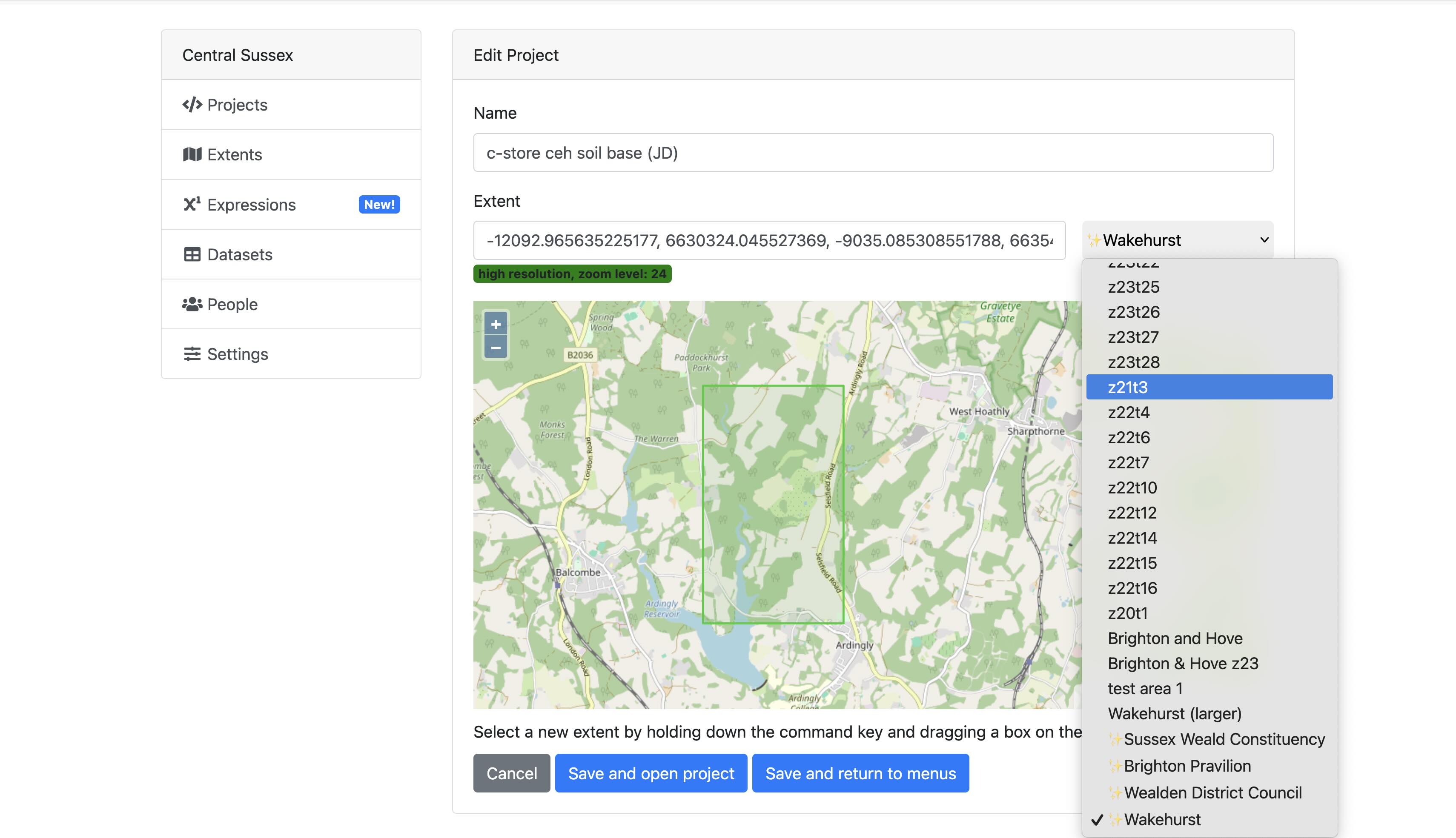
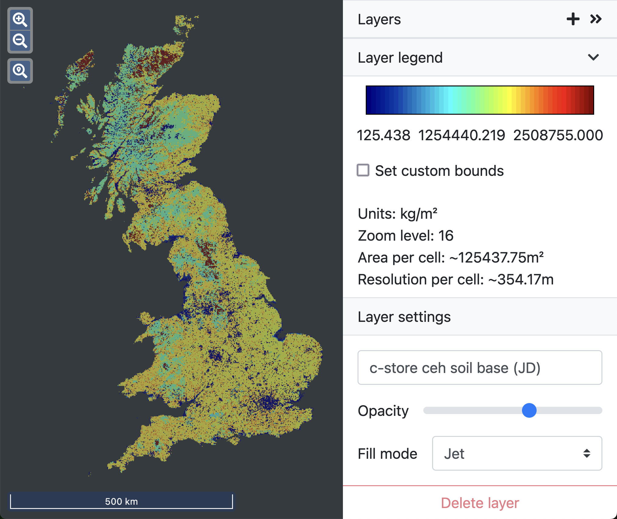
Due to the limitations of processing power, as the area analysed by the model increases the resolution of data used in the model decreases. This relationship is expressed in terms of ‘zoom levels.’ At the highest zoom level (24) each cell of the model is approximately 1.5 x 1.5 metres (with an area of around 2.25 m²) and a model at this resolution can be run over an area of around 6-7 km², an area the size of Wakehurst for example.
At zoom level 16 a model can cover the entire United Kingdom. In this case each cell of the model would be 354 x 354 metres and cover an area roughly 125,437 m² per cell.
This doesn’t mean, however, that a model cannot be run at a high zoom level (high resolution) across a wider area. It simply means that you would have to run the model multiple times across smaller areas and then stitch the results together in a separate project to view them on a single map. In this way you could generate a district or regional map at zoom level 24 without much difficulty.
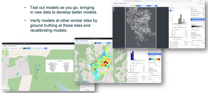
1.6 Extrapolation and Ground Truthing
As a research team you might want to use sample data to extrapolate estimates of various parameters of, for example, soil health and biodiversity indicators across your sampling area. Multi-parameter georeferenced point data from sampling can be used in LIMMMA’s Map View and Model View and the “Interpolation” component provides the capability to choose various interpolation methods using such point data to generate new map layers. This makes it possible to carry out ground truthing to callibrate models and to test their wider applicability beyond specific study sites.
1.7 Land-use Change Implications
Beyond mapping particular characteristics of landscapes (e.g. carbon storage, biodiversity, habitat fragmentation) or creating opportunity maps (e.g. for nature recovery options) LIMMMA can also be used to explore the potential implications of land use change over time.
At the regional or national scale we might consider the question, what if we planted more trees of a particular type in certain areas vs other areas? By using the outputs from models of carbon storage and biodiversity indicators alongside outputs from nature recovery opportunity maps as inputs into new models, it would be possible to estimate the potential impacts of various scenarios of nature recovery interventions across the landscape.
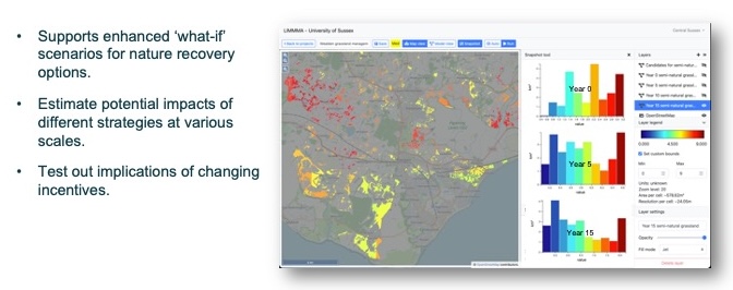
At the community level we might be interested to compare local urban and commercial development plans against nature recovery opportunity maps generated by local communities. We could then incorporate outputs from other landscape models to estimate the combined effects of land use strategies on environmental and social outcomes.
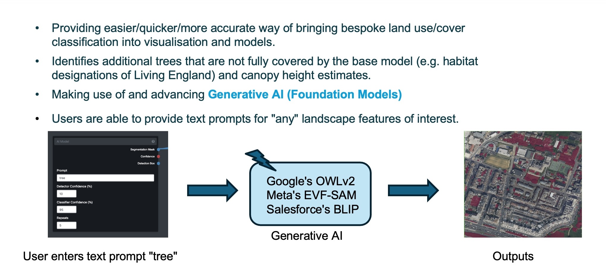
1.8 AI-assisted Land-use Land-cover Mapping
LIMMMA has a built in AI component to allow the user to create bespoke land-use land-cover maps by using machine learning to identify specific landscape features from satellite and aerial imagery. This can be particularly helpful for enhancing the habitat maps and land-cover base maps used in modelling with LIMMMA. For example, the AI component can identify lone trees and urban street trees which aren’t recognised by the LE or UKCEH habitat maps and it can distinguish between designated “green space” which does or does not have real vegetation cover (such as urban gardens and driveways).
1.9 Composite Models for Multifunctional Landscape Analysis
One further feature of LIMMMA which increases its flexibility and power is the ability save and reuse model outputs as datasets for use in new composite models. This makes it possible to create new map layers which model the multiple implications of complex changes in land-use across a host of dimensions such as biophysical, social and economic. For example, in one model, estimates of carbon storage in soils and vegetation can be used to predict carbon flux while in another model, biodiversity sampling might be used to extrapolate biodiversity indicators and predict biodiversity gain for various types of nature recovery intervention. A separate model would analyse the fragmentation of particular key habitats and identify priority locations for habitat corridors and connectivity projects. A further model might identify areas of high deprivation and lack of access to green space to identify key targets for specific types of nature recovery projects. Bringing together the outputs from each model into a composite model would allow the user to estimate the potential impacts of changes in land-use over time across each dimension of interest.